Overview
Part 1: Masses and Springs
Part 2: Simulation via numerical integration
Part 3: Handling collisions with other objects
Part 4: Handling self-collisions
Part 5: Shaders
In this project, we will build a real-time cloth simulation using a mass and spring system as well as write a variety of shaders. Parts 1 through 4 detail the process for creating the cloth simulation, and Part 5 pertains to the shaders.
To represent a cloth, we will use the mass and spring model in which we construct a grid of evenly spaced masses and connect nearby masses with springs.
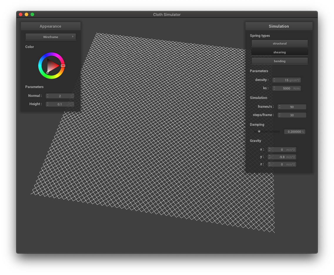
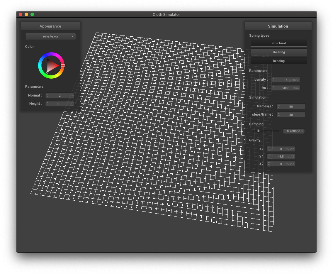
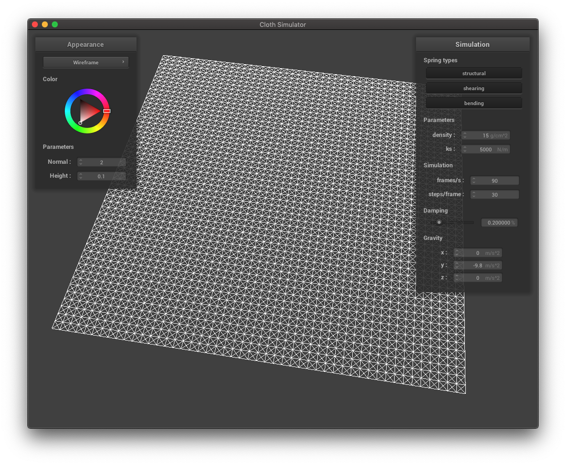
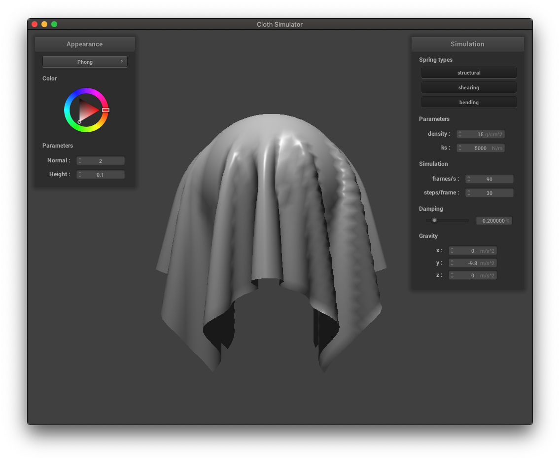
There are three types of constraints that can occur between point masses: structural, shearing, and bending. Each spring will apply one of these three constraints. Structural constraints exist between a point mass and the point mass to its left as well as the point mass above it. Shearing constraints exist between a point mass and the point mass to its diagonal upper left and the point mass to its upper right. Bending constraints exist between a point mass and the point mass two away to its left and the point mass two above it.
The images below depict the mass-spring grid with various spring types turned on or off.
Now that we have the mass-spring system that models the cloth, we want to simulate the cloth's movement by integrating the physical equations of motion. At each time step, forces are applied on the point masses and the point mass positions are updated.
The forces that need to be applied to the point masses are external forces (such as gravity) and spring-correction forces (which apply the spring constraints and are calculated using Hooke's law).
Then, to update the point mass positions, we will use the explicit integrator: Verlet integration. We will also add a damping term to simulate loss of energy due to friction, heat loss, etc. The point mass's new position \(x_{t + dt}\) is then given by $$ x_{t + dt} = x_t + (1 - d) \cdot (x_t - x_{t - dt}) + a_t \cdot dt^2$$ where \(x_t\) is the current position, \(d\) is the damping term, \(x_t - x_{t - dt}\) approximates \(v_t \cdot dt\) which is the current velocity times the timestep, \(a_t\) is the current total acceleration from all forces, and \(dt\) is the timestep.
Finally, we will add some additional position update constraints. In particular, we want to limit a spring's length to be at most 10% greater than its rest length. Therefore, if needed, we will correct the point mass positions of each spring so that this condition is met.
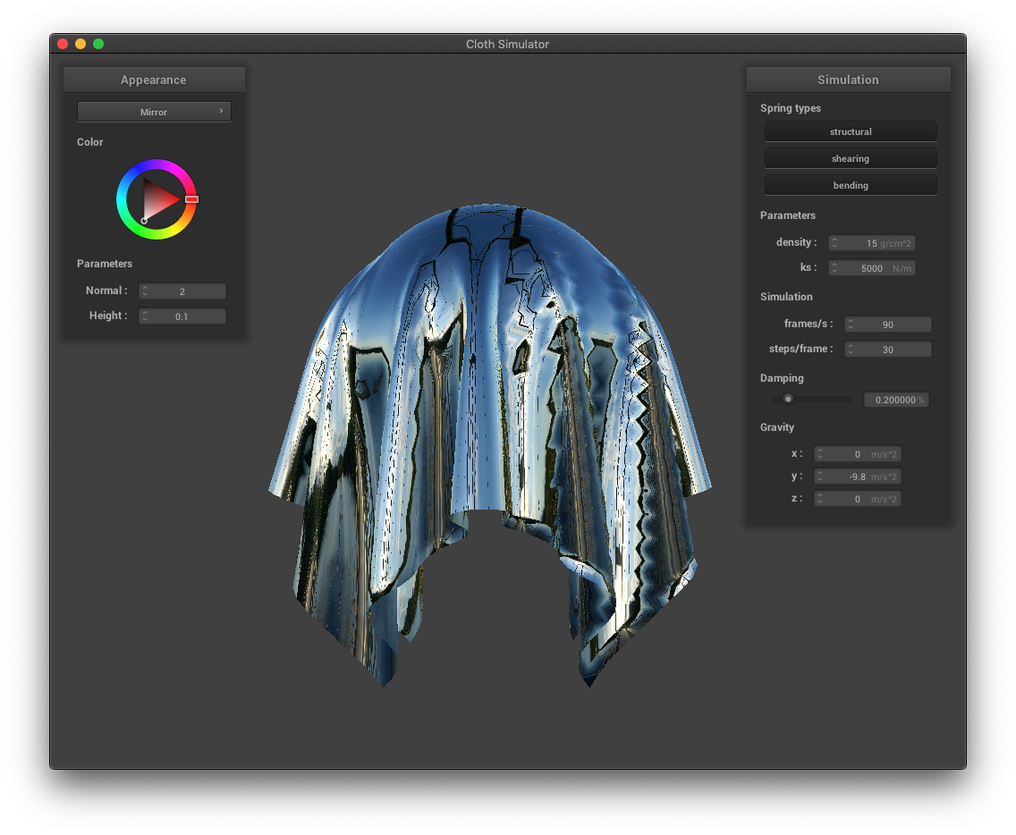
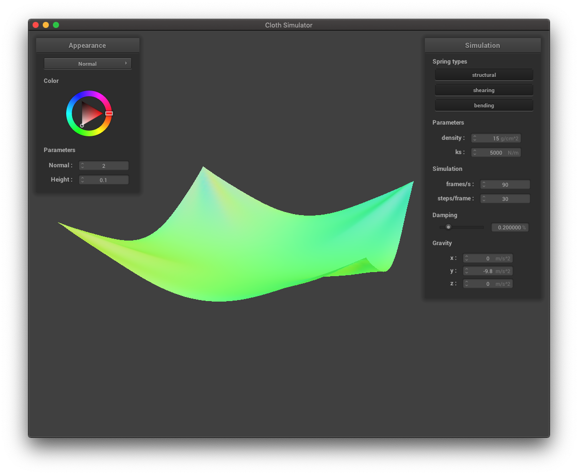
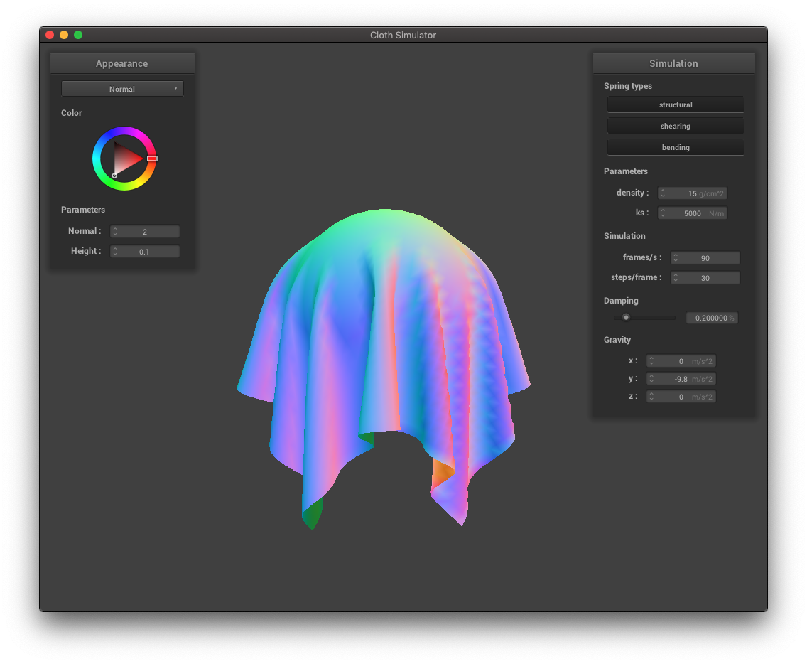
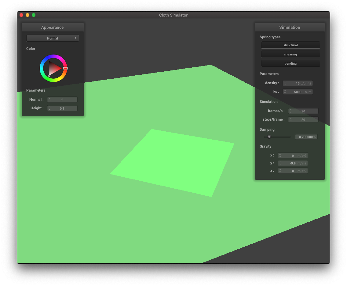
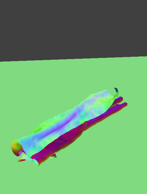
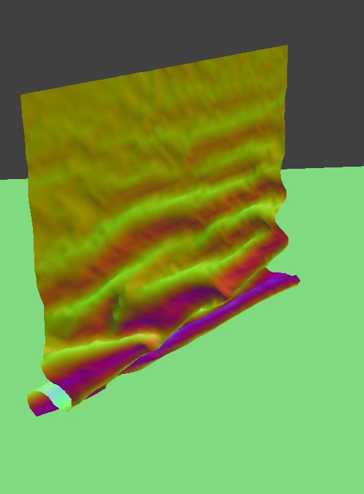
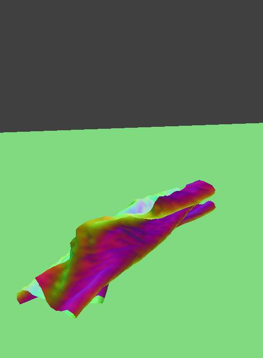
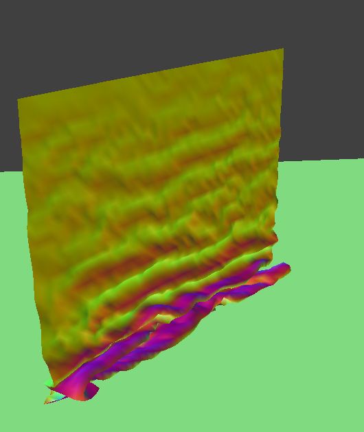
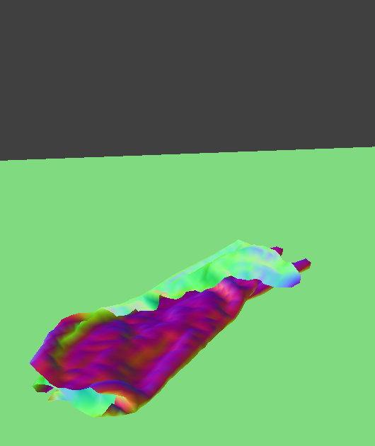
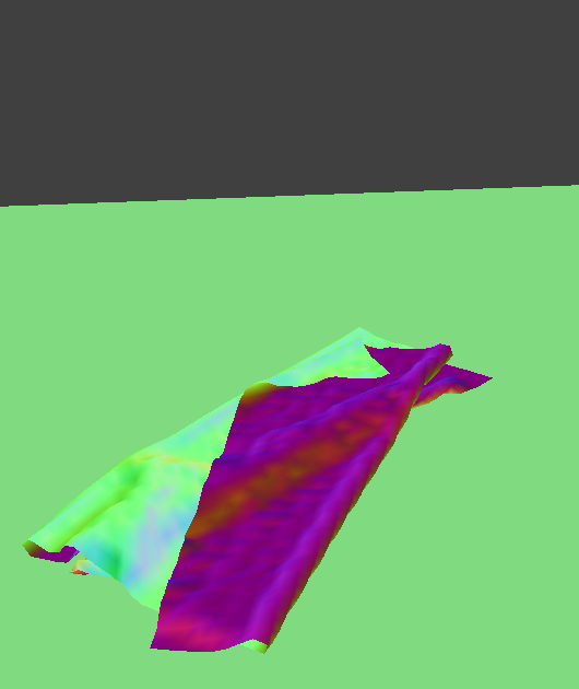
The two images below show the same cloth at its rest state after undergoing the simulation. We can visualize the mass-spring system with the Wireframe model and the folds of the cloth with Normal shading.
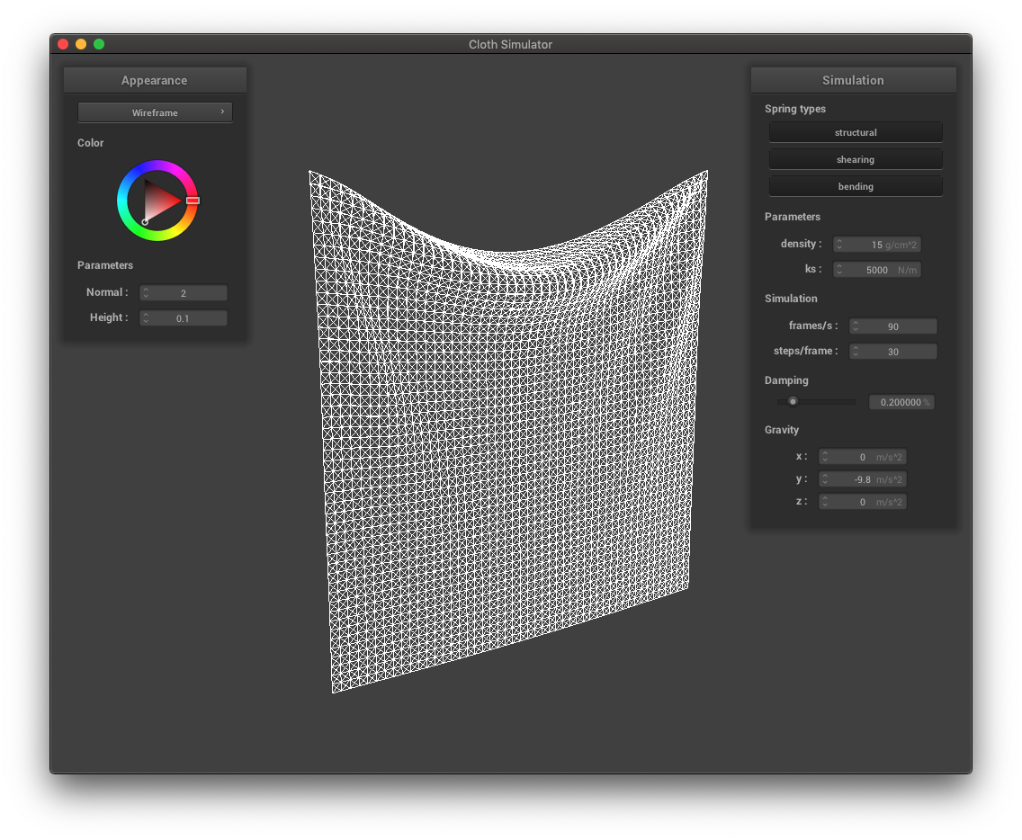
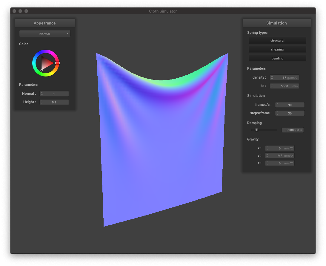
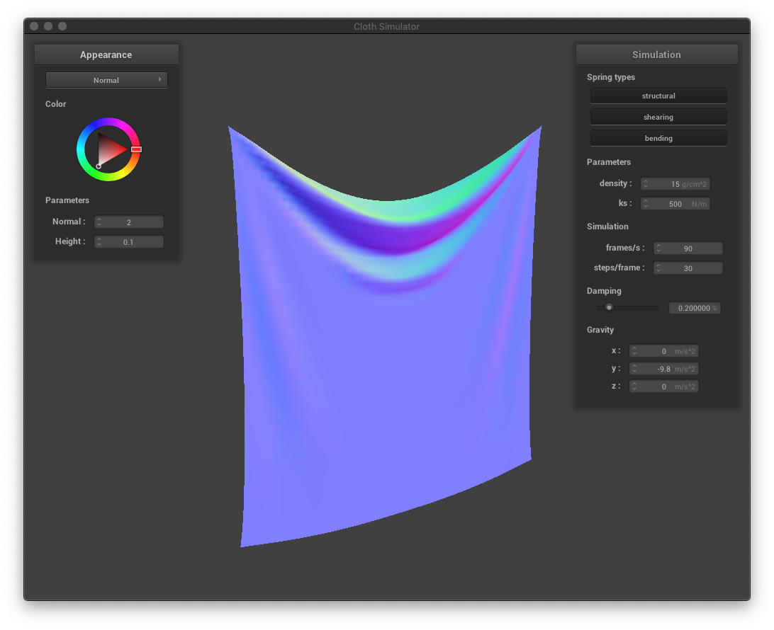
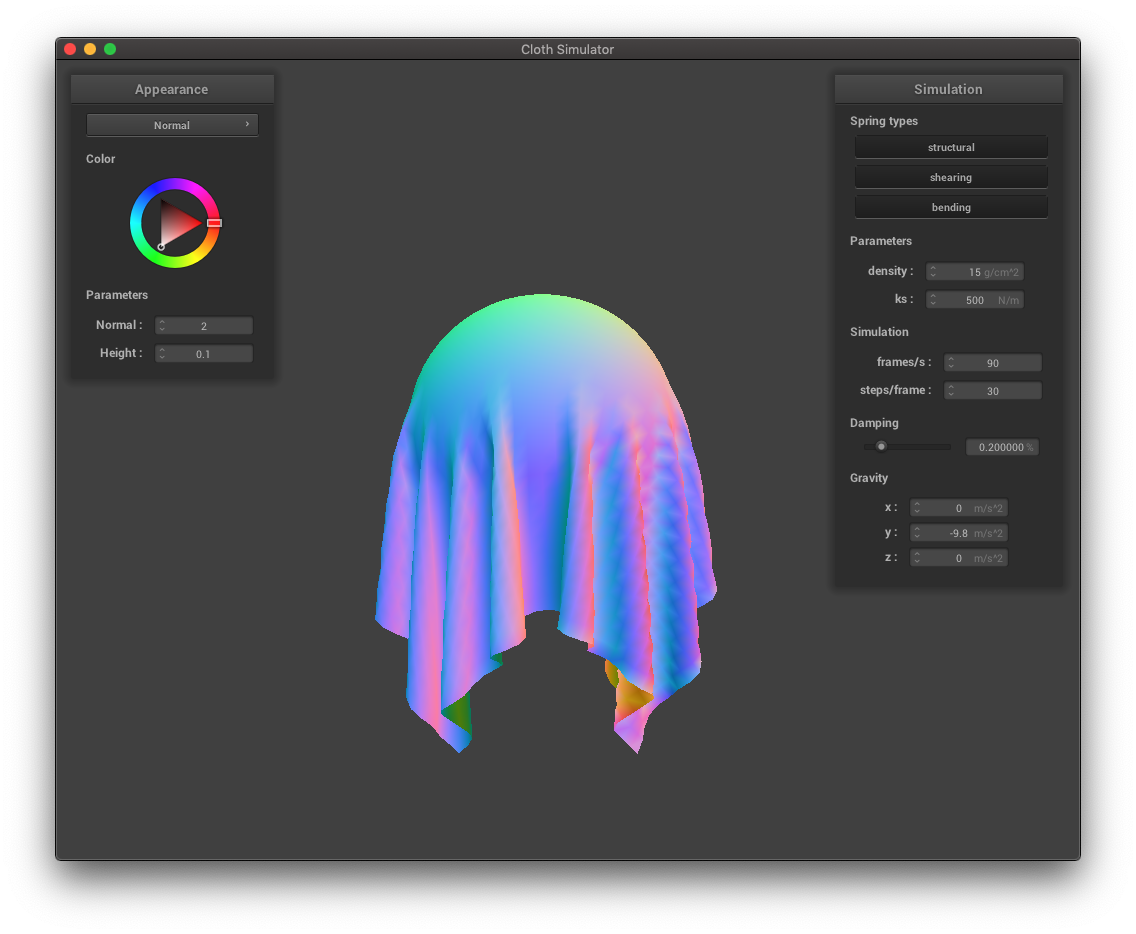
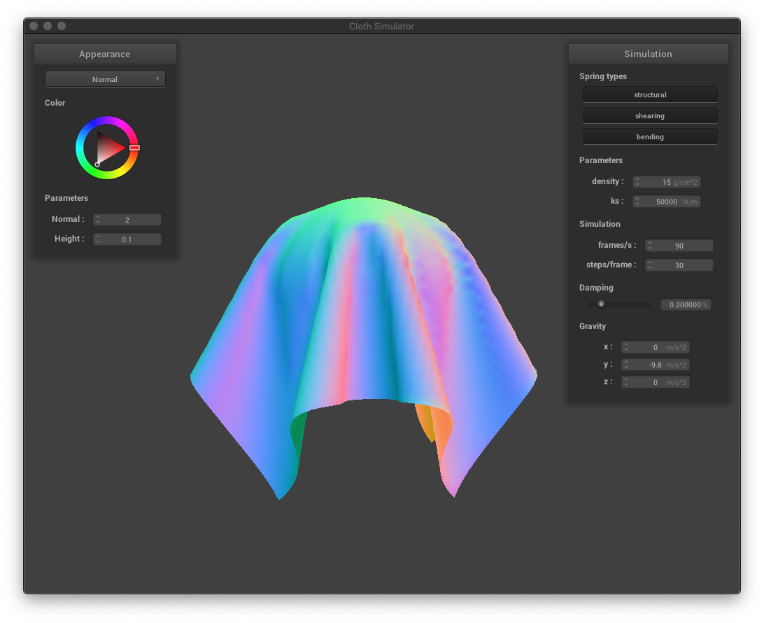
Changing the parameters of the simulation produces different results.
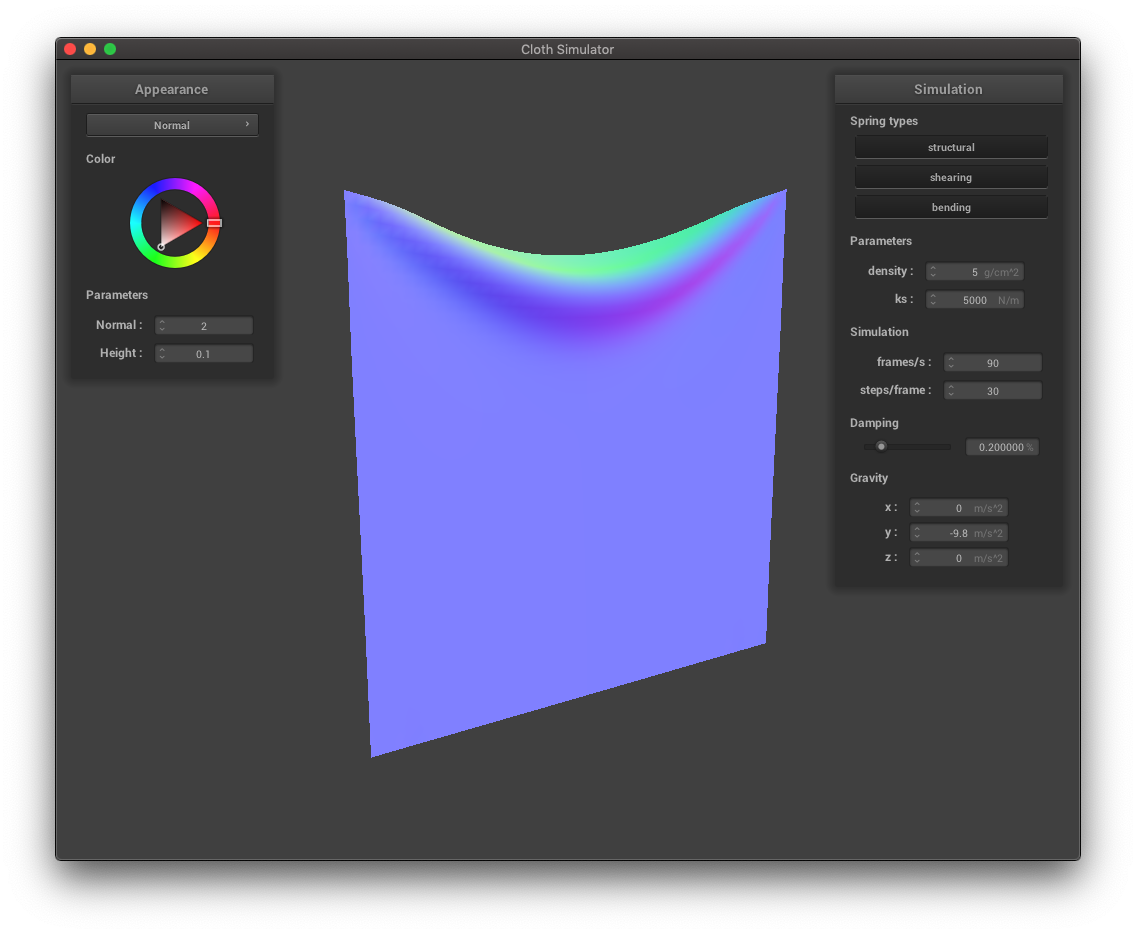
For example, a lower spring constant
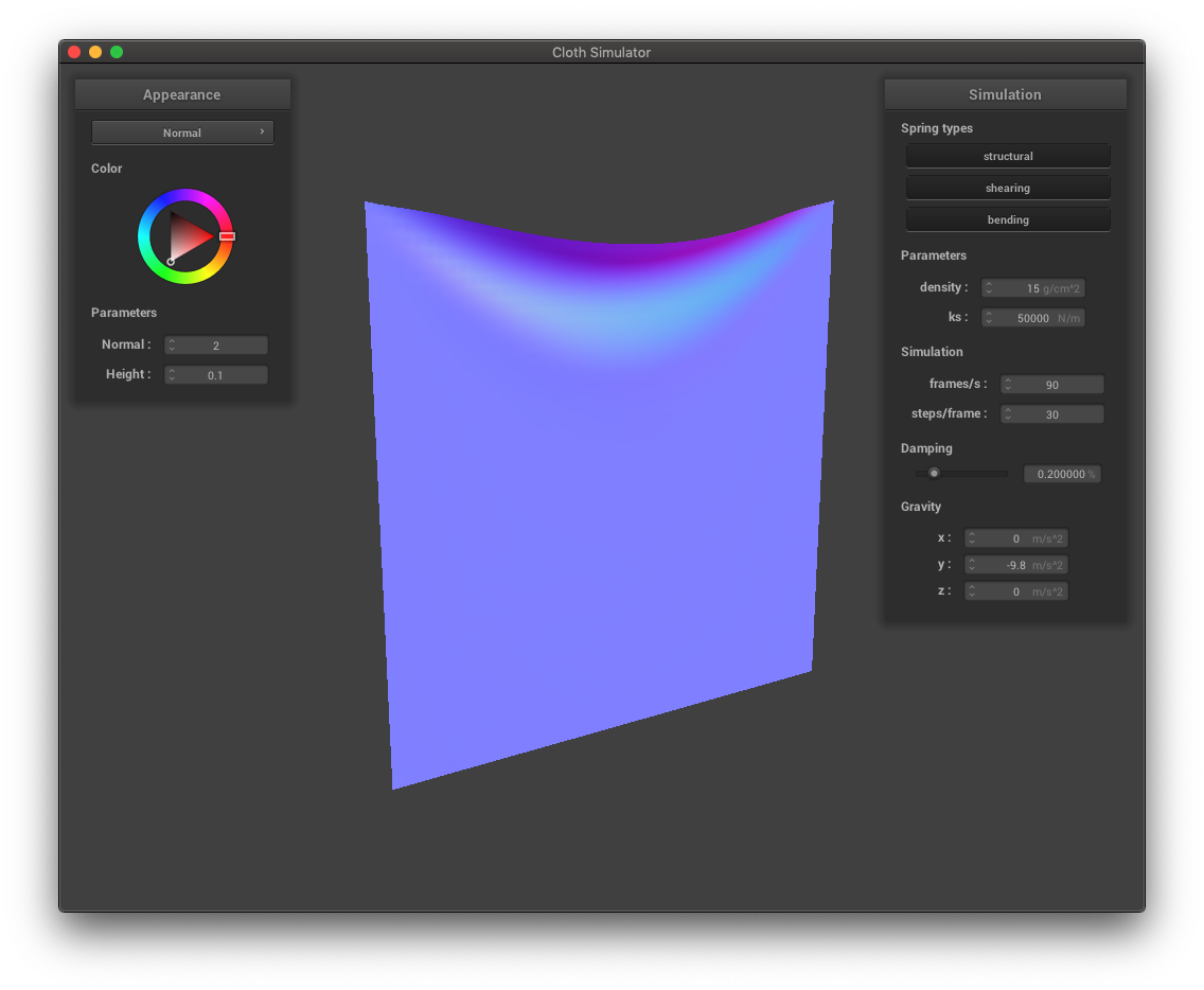
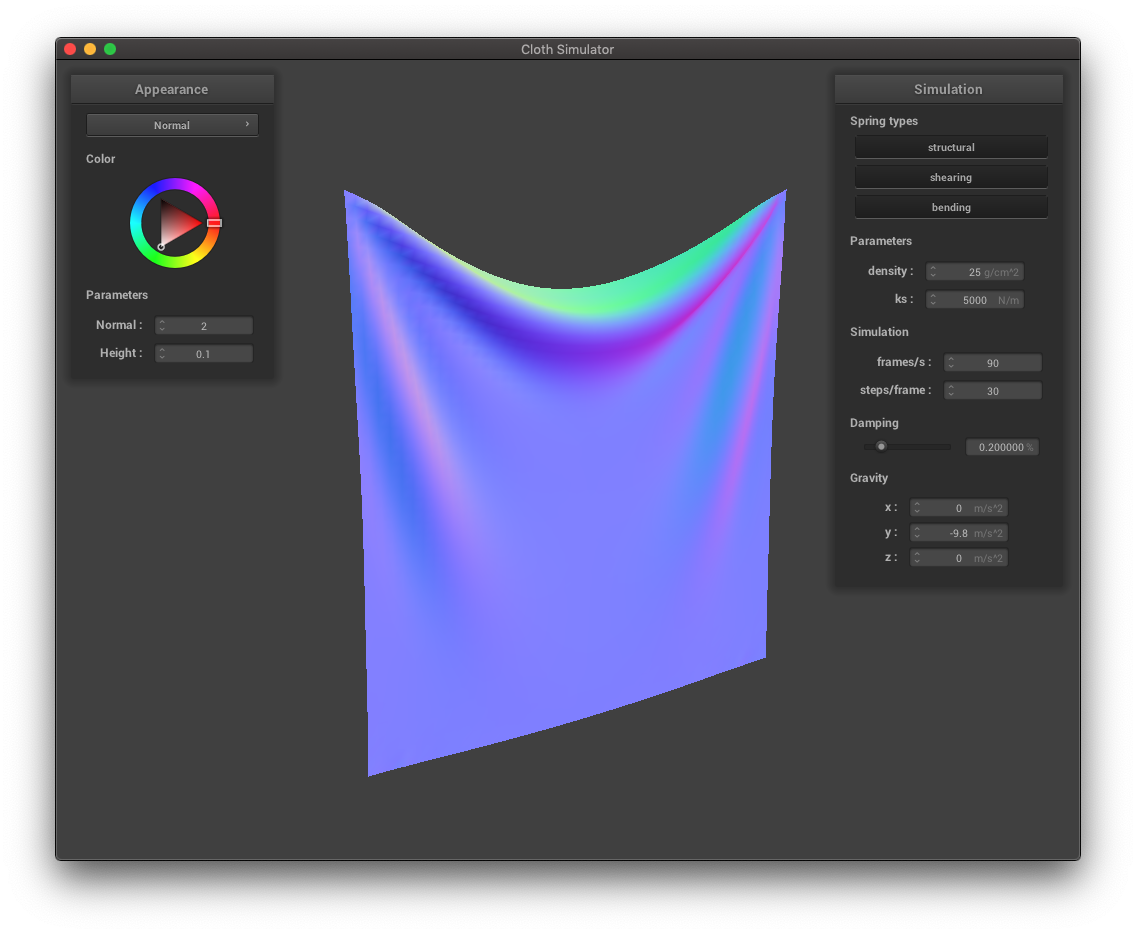
The density of the cloth also has an impact on its final rest state. Below, the higher density cloth is pulled downwards (by its own weight) more so than the lower density cloth.
The damping factor also plays a role in the cloth's behavior. As shown in the videos below, a higher damping factor will cause the cloth to end up at its rest state more directly. The cloth with a low damping factor moved back and forth before reaching its rest state.
Previously, we were able to simulate how a cloth drapes when pinned at certain corners. Now, let's see how the cloth interacts with other objects by simulating collisions with other objects.
We will add support for cloth-sphere and cloth-plane collisions. The general idea is: when any point mass's position intersects/enters an object, we will correct the position and "bump" it back to the surface of the object.
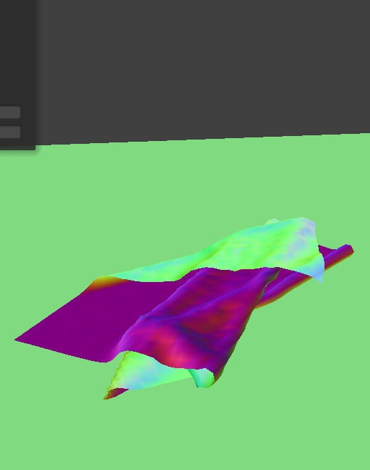
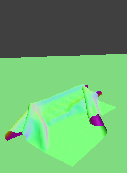
The following show a piece of cloth draped over a sphere and a piece of cloth at rest on a plane.
Again, we can adjust the cloth parameters such as the spring constant. As depicted below, a lower spring constant gives the appearance of a thinner, stretchier material while the higher spring constant makes the cloth look stiff. The cloth-sphere collision image from above uses a spring constant of 5000 N/m, so its stiffness lies between those of the two cloths below.
One issue that we may have encountered in the previous parts is the cloth clipping through itself. Adding support for self-collisions will fix this behavior.
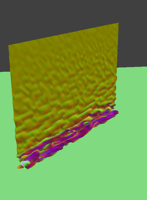
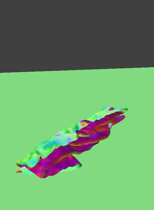
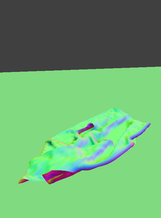
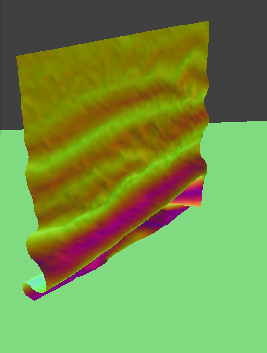
In each of the following groups of three images, a cloth is shown at its early stage of falling, its middle stage, and its final resting state. The cloth below uses the default parameters.
Like how we did in previous parts, we can adjust these parameters to produce simulations that exhibit different cloth behaviors. A low spring constant allows for more fine wrinkles, so the final resting state of the low spring constant cloth is more "bunched up". On the other hand, the high spring constant cloth has far less wrinkles and flattens out as it reaches its resting state.
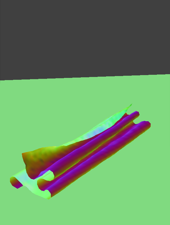
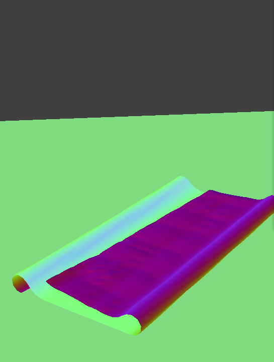
Changing the density of the cloths does not have as dramatic of a difference. A slight difference is in how "open" the folds of each cloth are. The low density cloth has wider and more "open" folds, mainly visible in the early stage and resting state images. The high density cloth has flatter folds in comparison, most noticeable in the resting state image.
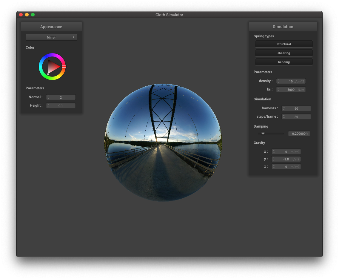
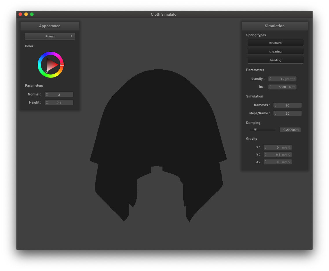
Now that we have a cloth simulator, let's build some shaders so that we can visualize the cloth in a variety of ways. We will write diffuse, blinn-phong, texture mapping, bump mapping, displacement mapping, and mirror shaders. A shader is a program that runs in parallel on the GPU, letting us render materials for real-time applications such as our cloth simulation. We will write our shaders in GLSL and use OpenGL vertex and fragment shaders. Vertex shaders apply the transforms to the vertices and modify geometric properties. Fragment shaders take in geometric attributes (calculated by the vertex shader) and output a color. Corresponding vertex and fragments shaders are linked together to form the shader program: the output of the vertex shader is the input to the fragment shader.
The Blinn-Phong shading model is comprised of multiple components: ambient light, diffuse light, and specular reflection. The overall Blinn-Phong reflection is a sum of these three components. This is shown in the following equation
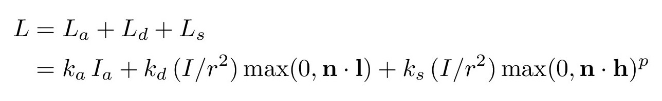
Credit: CS184/284A Lecture 6 Slides by Ren Ng
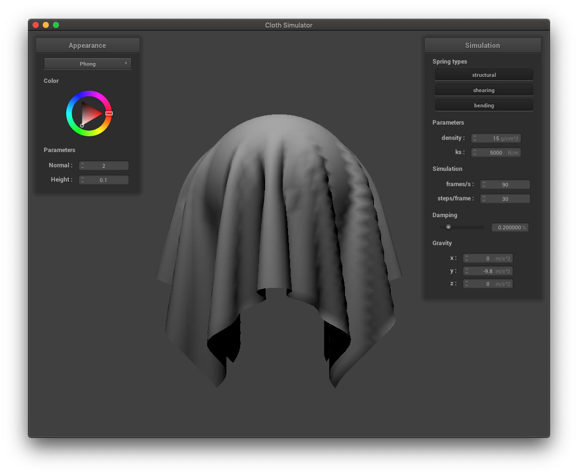
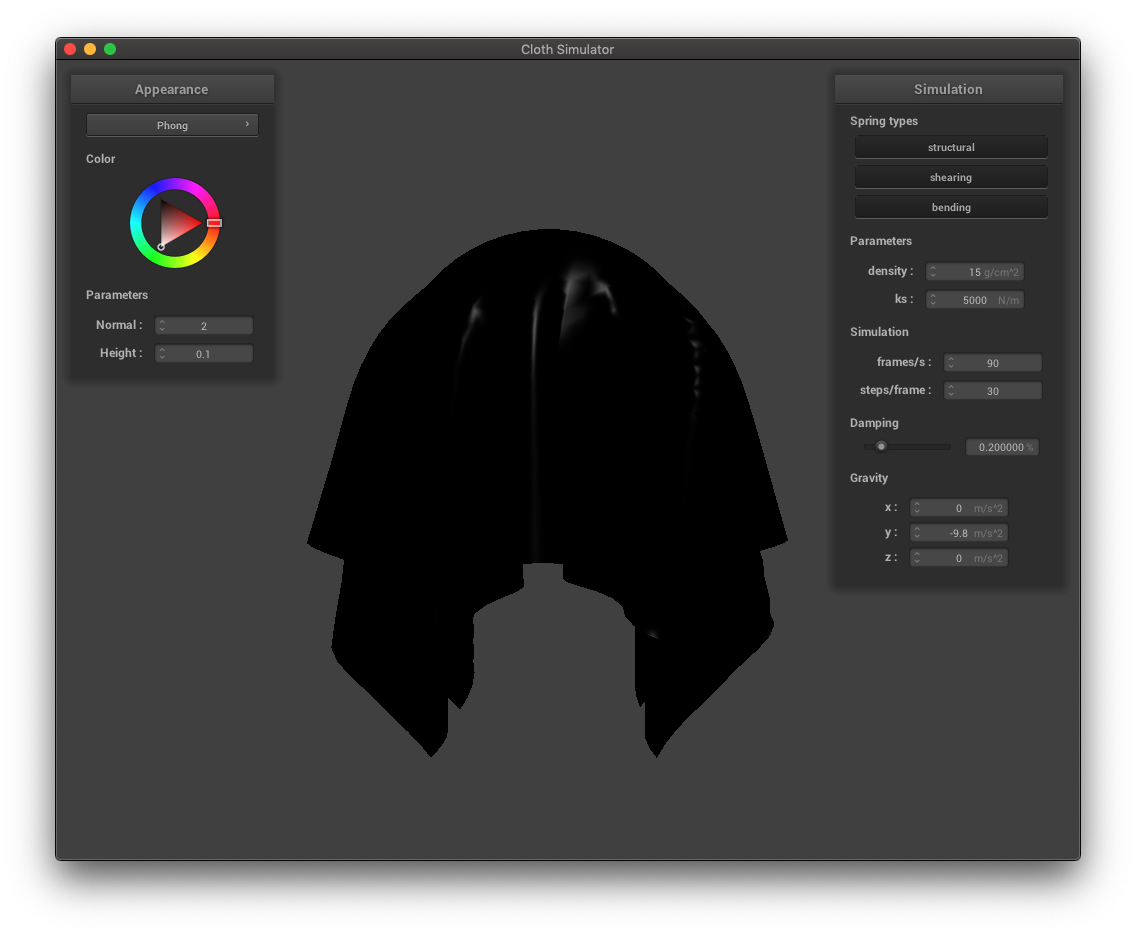
Each of the three components (as well as the full Blinn-Phong shading model) are illustrated below.
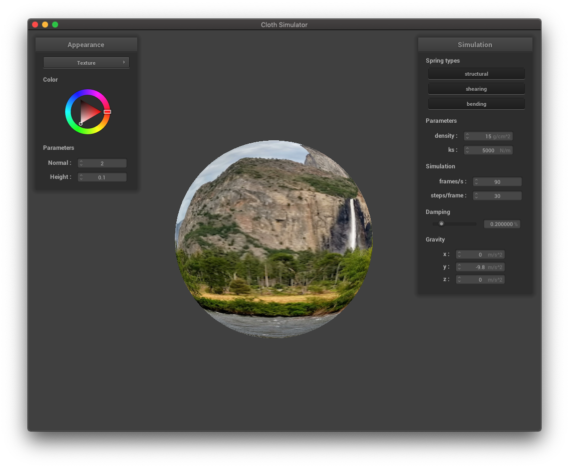
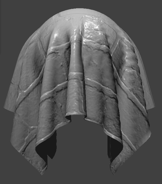
We can also map a texture onto the cloth and sphere as shown below.

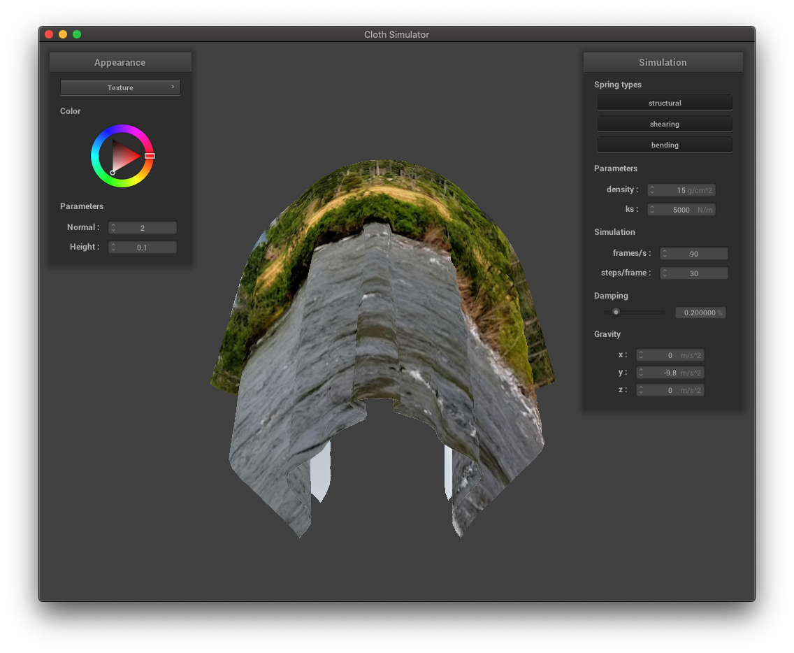
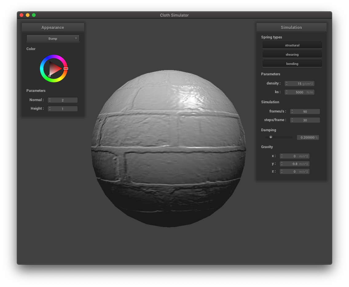
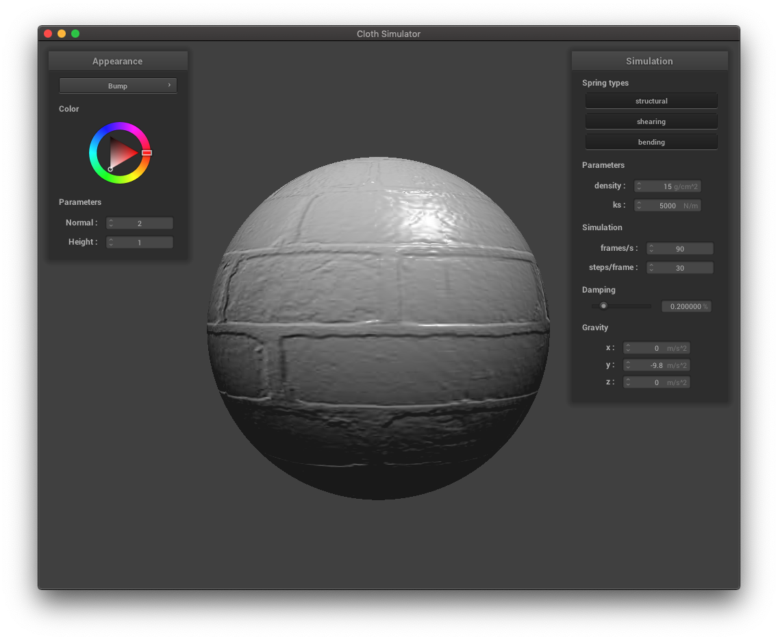
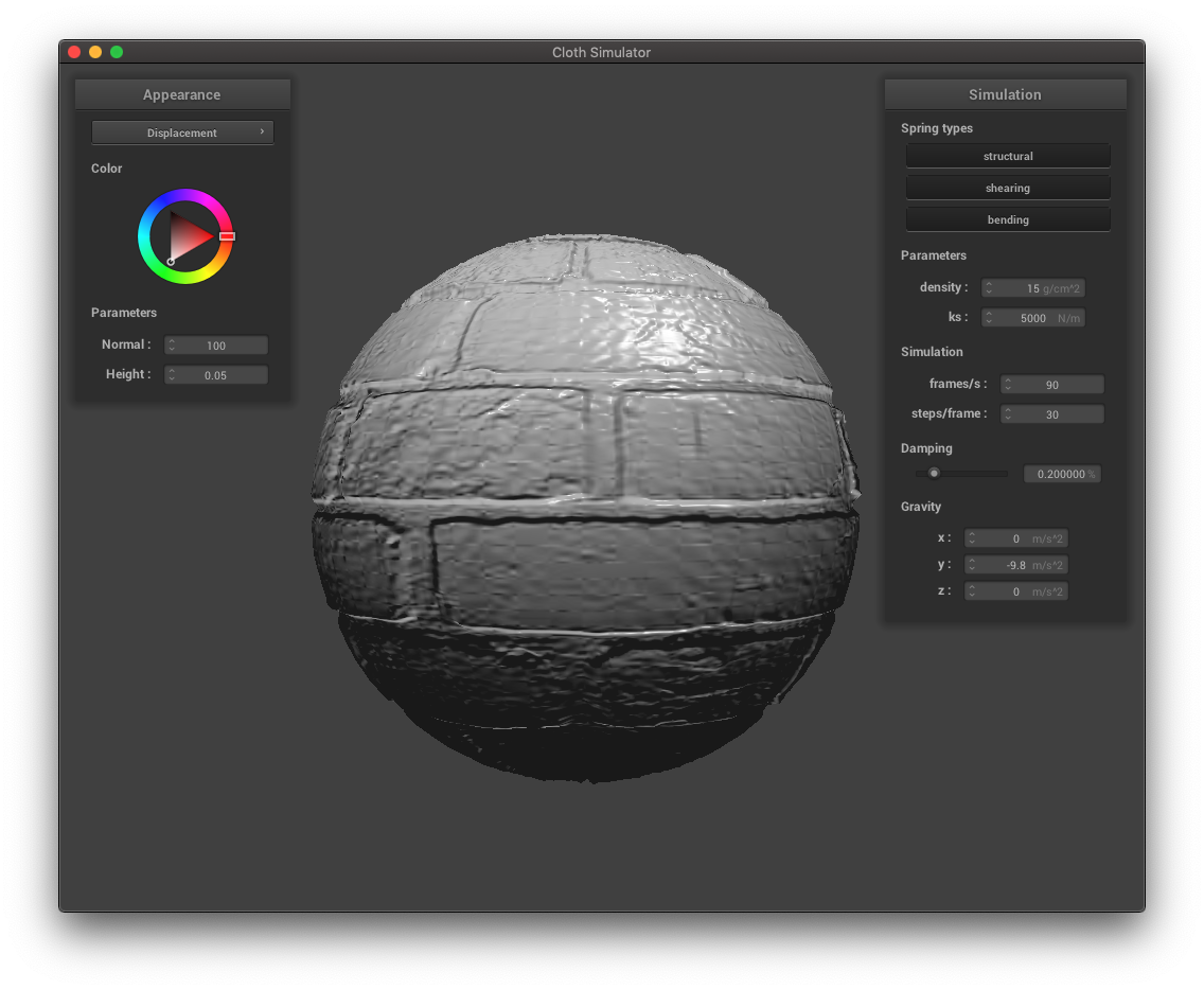
Bump mapping will give the illusion of a heightened surface but it won't actually change any vertex positions. This is apparent when we view the "edges" of the sphere which are still smooth. In contrast, displacement mapping will actually change vertex positions. Now, if we look at the "edges" of the sphere, we can see the 3D displacement of the textured surface.
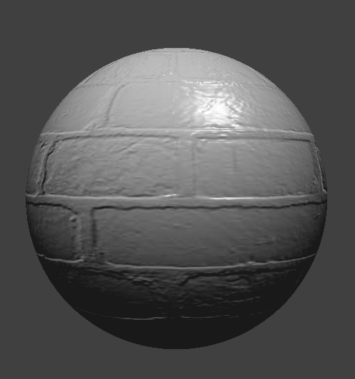
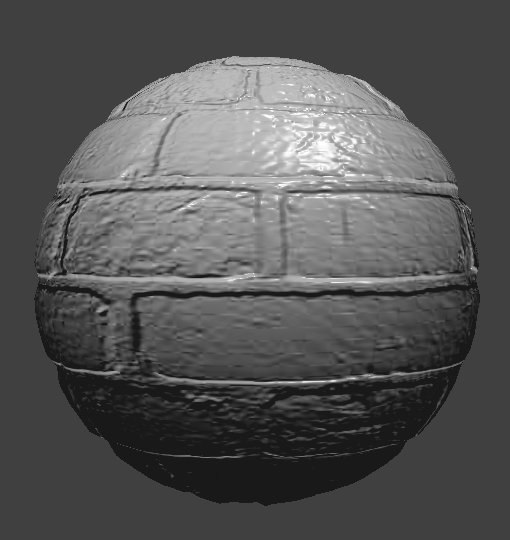
For both the low and high resolution spheres, the bump mapping shaders look fine. But when we start to make changes to the geometry, as the displacement mapping shader does, the resolution starts to matter. The resolution has an impact on how well the displacement mapping shader performs because there needs to be enough geometry for the shader to work with. Otherwise, the sphere "edges" appear blocky. In the upper right sphere (resolution = 16), the resolution is not high enough to cleanly define the textured surface displacement. We can see that this is fixed in the high resolution displacement mapping sphere, however.