Project 3-1: PathTracer

CS 184: Computer Graphics and Imaging, Spring 2022

Monica Tang

Table of Contents:

  Overview
  Part 1: Ray Generation and Scene Intersection
  Part 2: Bounding Volume Hierarchy
  Part 3: Direct Illumination
  Part 4: Global Illumination
  Part 5: Adaptive Sampling

Overview

This project explores topics such as ray-scene intersections, acceleration structures, and physically based lighting and materials. In each part, a core routine of the renderer is implemented, culminating in a physically-based renderer that uses a pathtracing algorithm to produce realistic images.

Part 1: Ray Generation and Scene Intersection

Ray Generation

In this part, we want to be able to generate rays and calculate where they intersect the primitives (e.g. triangle, sphere) in the scene.

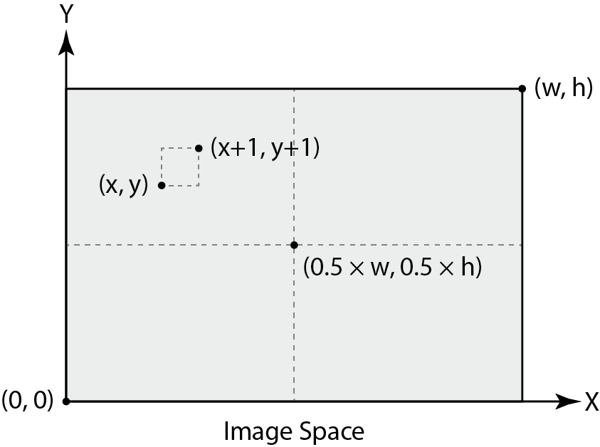
Given normalized \((x, y)\) image coordinates in image space, we want to transform them first into camera space and then into world space in order to generate rays. As described in the equations and image below, \((x, y)\) in image space is mapped to \((x', y')\) in camera space. $$x' = (x - 0.5) \cdot 2 \cdot \tan \Big(\frac{\text{hFov}}{2} \Big)$$ $$y' = (y - 0.5) \cdot 2 \cdot \tan \Big(\frac{\text{vFov}}{2} \Big)$$

Once we have the coordinates in camera space, we then create a ray. A ray has an origin and direction, both in world space. So, the ray we create has its origin at the camera position and its direction as \((x', y', -1)\) that is transformed to world space using a camera-to-world transformation matrix.

Then, to raytrace a pixel, we calculate the Monte Carlo estimate of the integral of radiance over the pixel by taking multiple samples within the pixel and averaging their radiances. The figure below shows a pixel at unnormalized pixel coordinates \((x, y)\).

Scene Intersections

Now that we have generated rays, we can use intersection algorithms to detect where a ray intersects a primitive in the scene. We will explore ray-triangle and ray-sphere intersection algorithms.

The Möller-Trumbore algorithm is a ray-triangle intersection algorithm that tells us the t-value (\(t\)) of the ray where the intersection occurs as well as the barycentric coordinates \((1 - b_1 - b_2, b_1, b_2)\) of the triangle where the intersection occurs. The math is as follows, where \(O + tD\) is the ray and \(P_i\) are the vertices of the triangle:

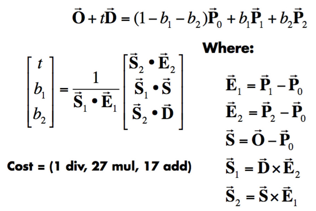
Credit: CS184/284A Lecture 9 Slides by Ren Ng, Angjoo Kanazawa

Calculations for finding the ray-sphere intersection t-value is defined in the following figure:

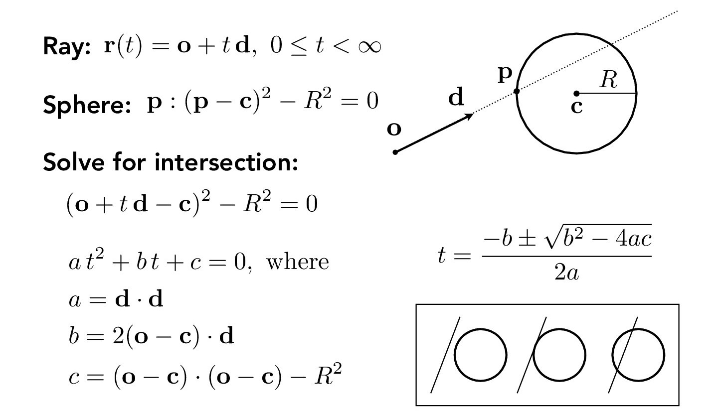
Credit: CS184/284A Lecture 9 Slides by Ren Ng, Angjoo Kanazawa

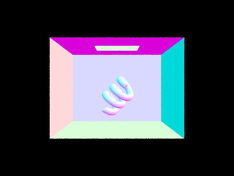
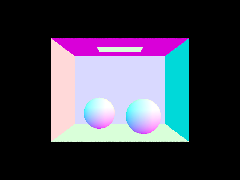
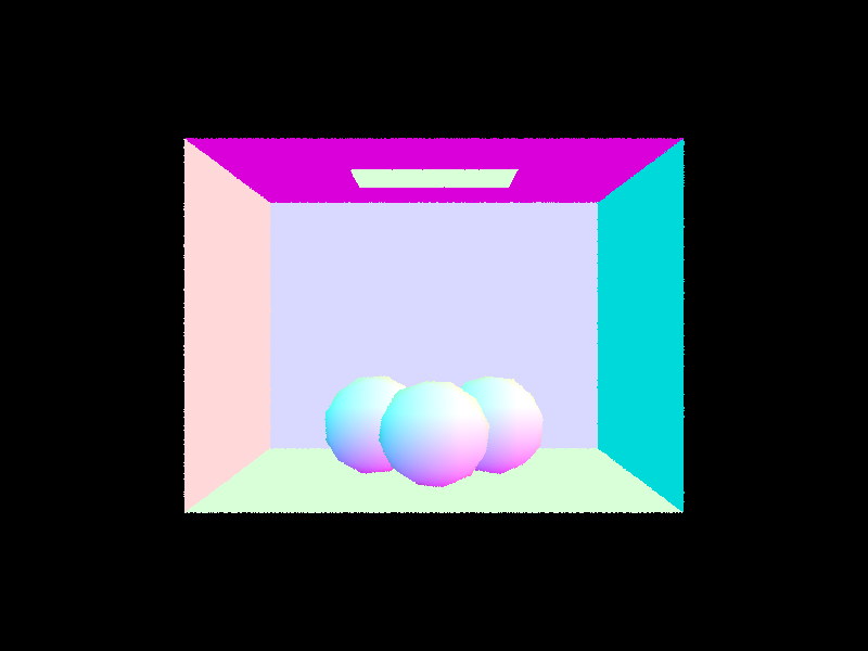
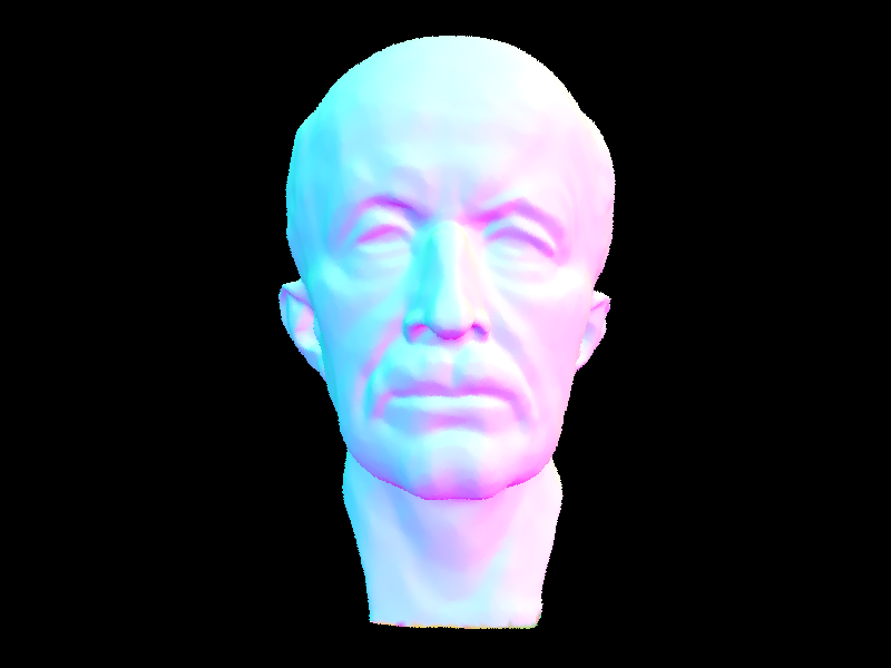
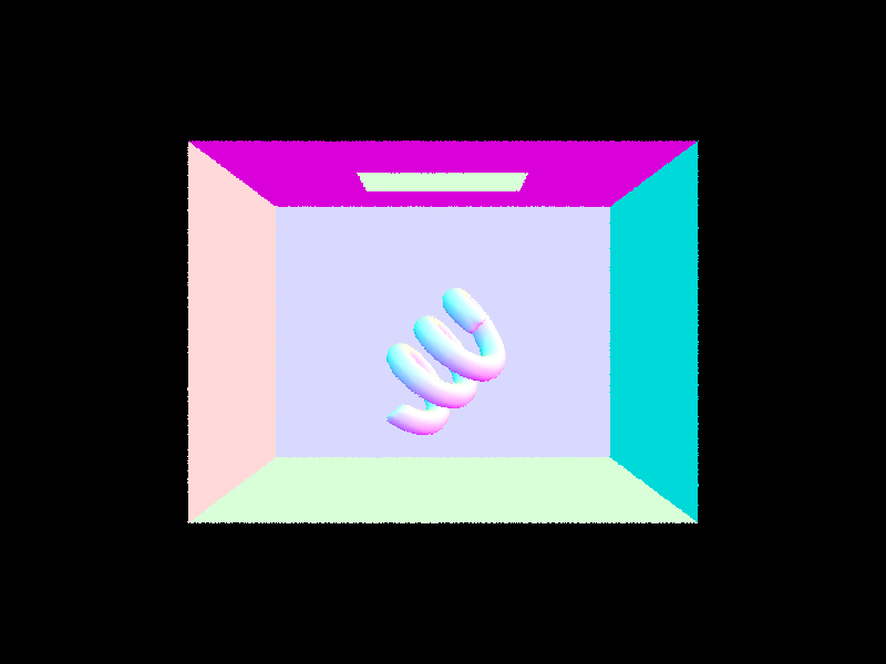
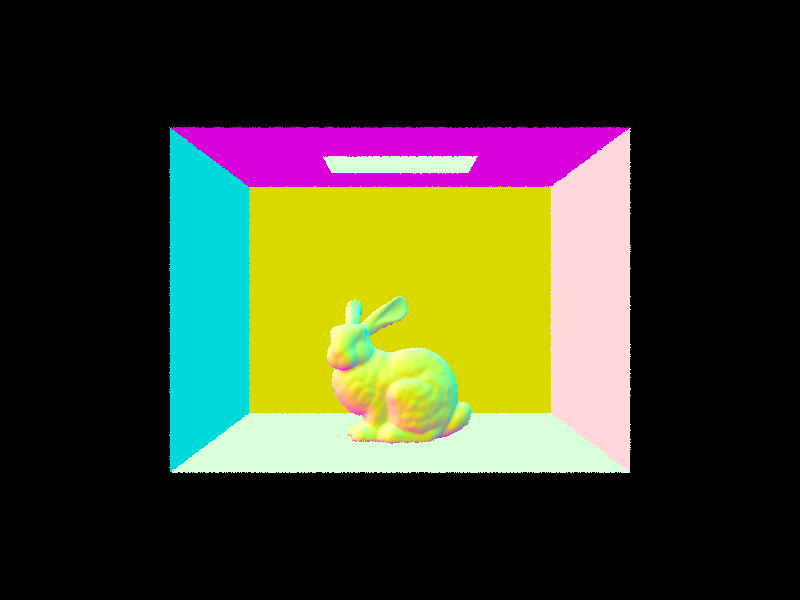
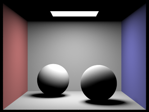
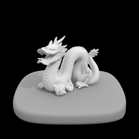
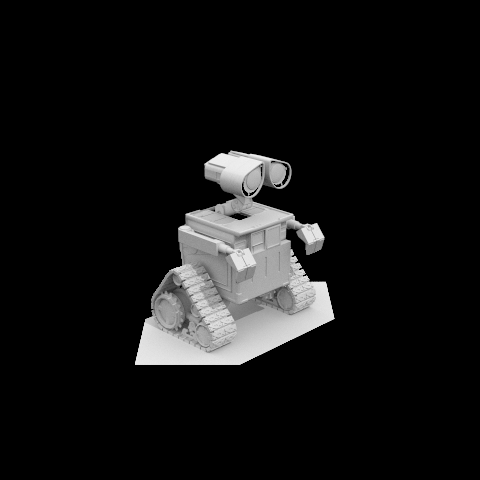
After implementing these features, we are now able to render geometry in scenes. Below are several examples.

Part 2: Bounding Volume Hierarchy

To render the scenes in Part 1, for each ray, we check if it intersects each primitive in the scene which is computationally heavy and time consuming. As a result, we're unable to render more complex scenes in reasonable times. This motivates the Bounding Volume Hierarchy (BVH) which improves the efficiency of the renderer.

The BVH is a binary tree consisting of internal nodes (that store bounding box and children information) and leaf nodes (that store bounding box information and a list of the bounding box's primitives). The figure below is a simple illustration of this idea; the white nodes represent internal nodes, the colored/labeled nodes represent leaf nodes, and the gray rectangles represent the bounding boxes.

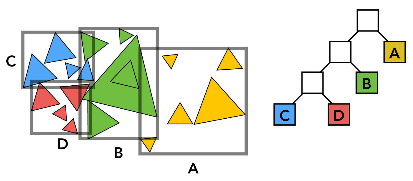
Credit: CS184/284A Lecture 10 Slides by Ren Ng

A key part in BVH construction is the splitting heuristic, which is used to determine which primitives go to the left and right children of a node. These are the steps I took to find a splitting point:

1. Choose the longest axis of the bounding box as the axis to split across.
2. Sort each primitive by centroid position in increasing order.
3. Split in half: left half goes to the left child, right half goes to the right child.

We then recurse on the left and right children and continue splitting the primitives into smaller and smaller bounding boxes. We stop when there are at most max_leaf_size primitives in a node.

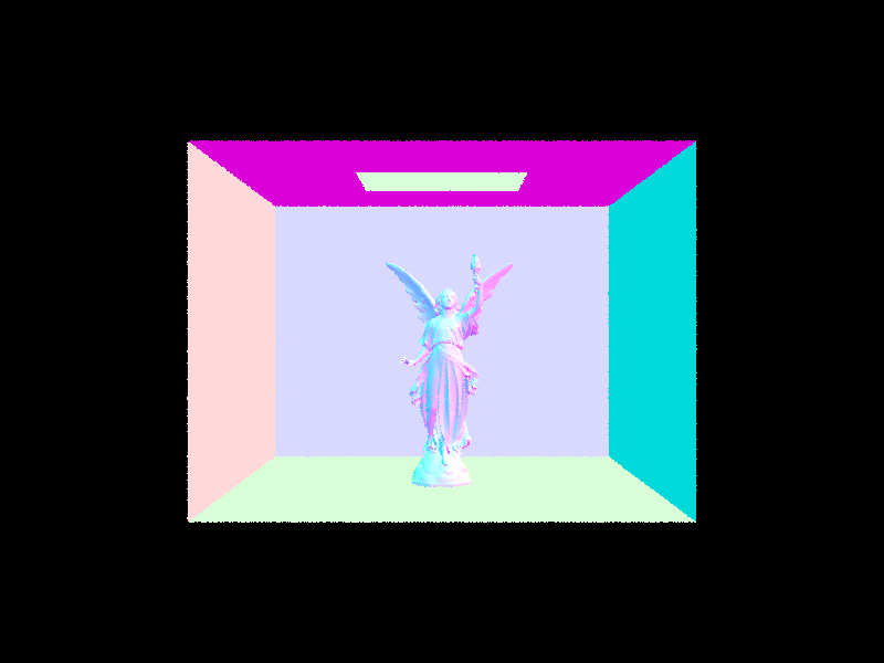
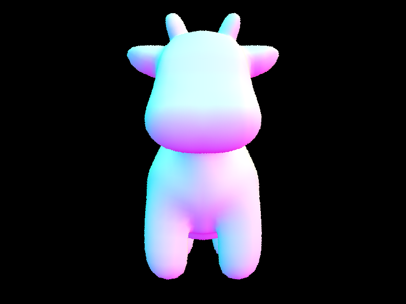
To use the BVH acceleration structure, when we trace a ray, we first check if the ray intersects a node's bounding box. If not, we don't bother with ray-primitive intersections in that bounding box. If so, we recurse on the left and right children of the node. Only until we reach a leaf node do we perform ray-triangle or ray-sphere intersection tests. This approach greatly improves the efficiency of rendering scenes and allows us to render complex scenes (like those below) that were not possible before.

Because of this efficiency, the BVH acceleration structure also results in substantial decreases in render times, which are indicated for each example below. In the cow.dae and CBcoil.dae files, using a BVH gives a ~185 - 300x speedup. For a slightly more complex scene such as CBbunny.dae, the speedup is even more drastic, around a 1000x speedup. This goes to show how much more efficient a BVH acceleration structure is than a single bounding box structure.

Part 3: Direct Illumination

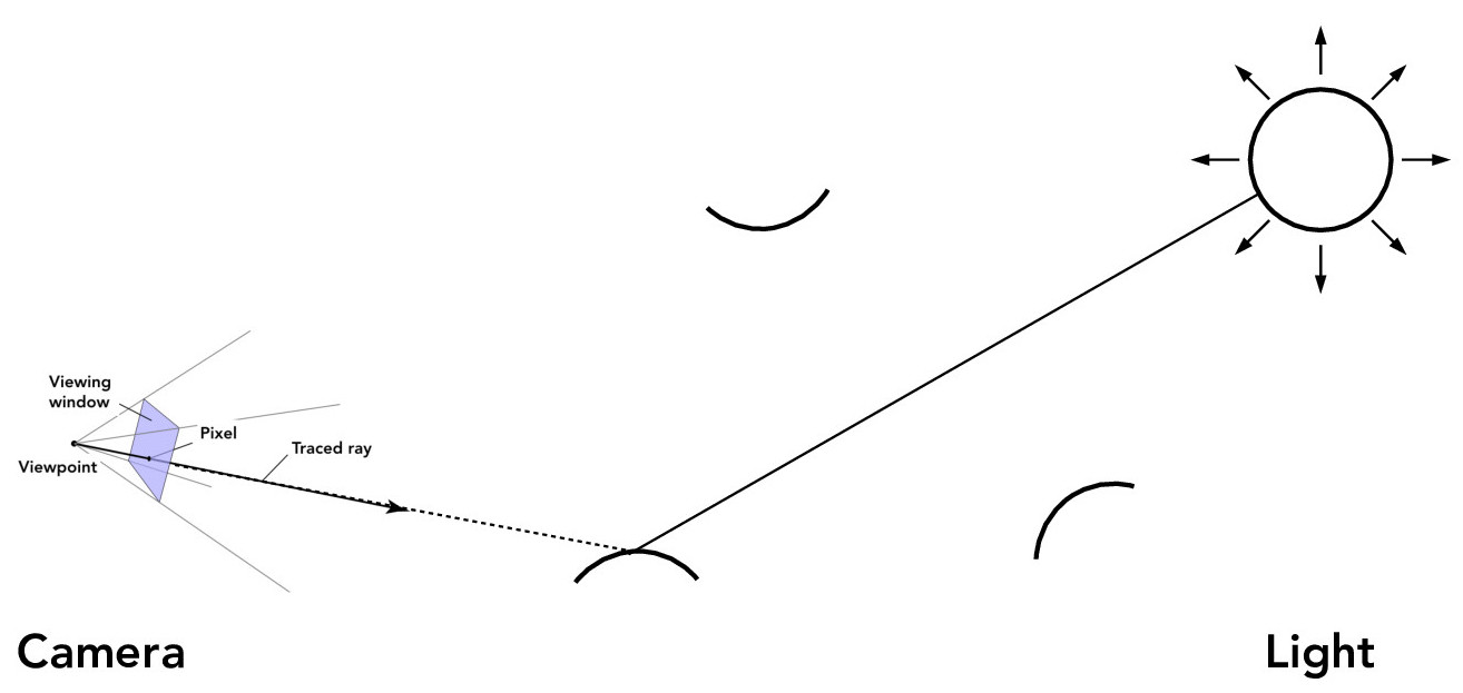
Now, we'd like to render our scenes with lighting. We will start with direct illumination which consists of zero bounce and one bounce illumination. Zero bounce illumination is simply the light that is emitted from the light sources directly to the camera without bouncing off of anything in the scene since non-light sources do not emit light and thus do not contribute to the total radiance. One bounce illumination refers to light that bounces once in the scene before reaching the camera.

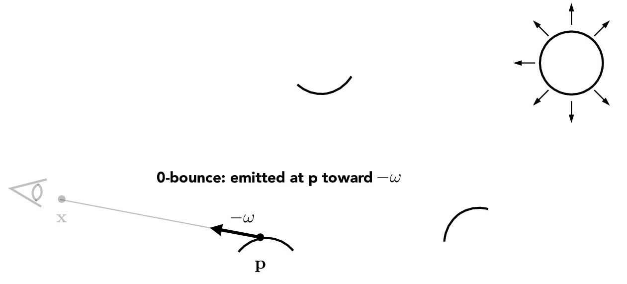
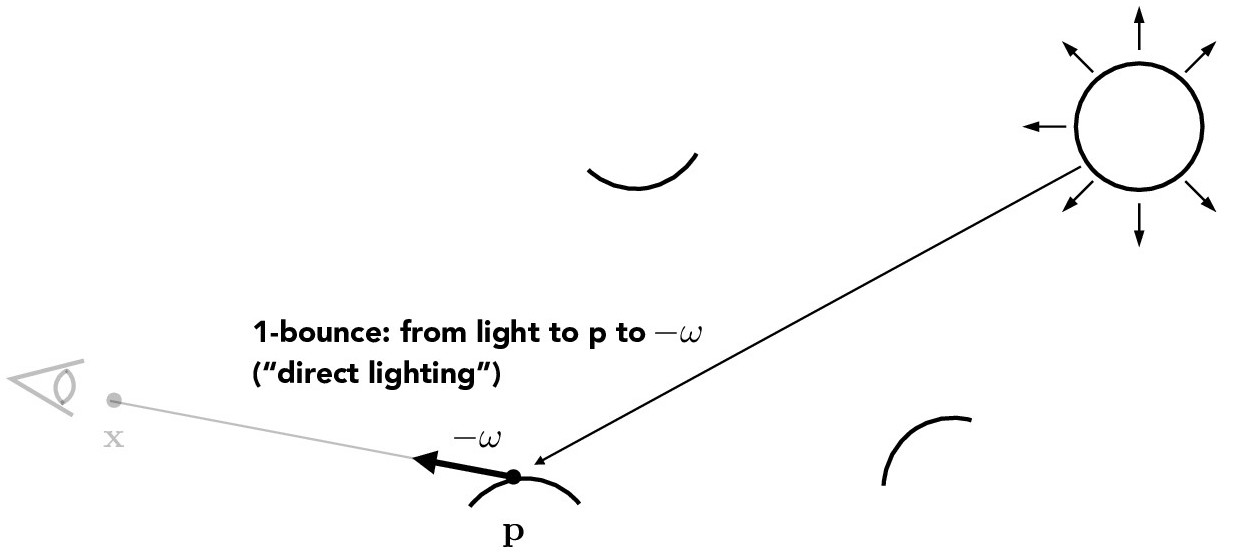
Credit: CS184/284A Lecture 13 Slides by Ren Ng

For efficiency's sake, we will trace inverse rays, which means we cast a ray from the camera, through a pixel, into the scene. Then, at the ray-scene intersection point, we calculate the light that is reflected back toward the camera.

Credit: CS184/284A Lecture 13 Slides by Ren Ng

The figures below describe the Reflectance Equation (which we approximate using a Monte Carlo estimator) and the BRDF function. In this project, we will only use Diffuse BRDFs, which reflect light equally in all directions on the hemisphere.

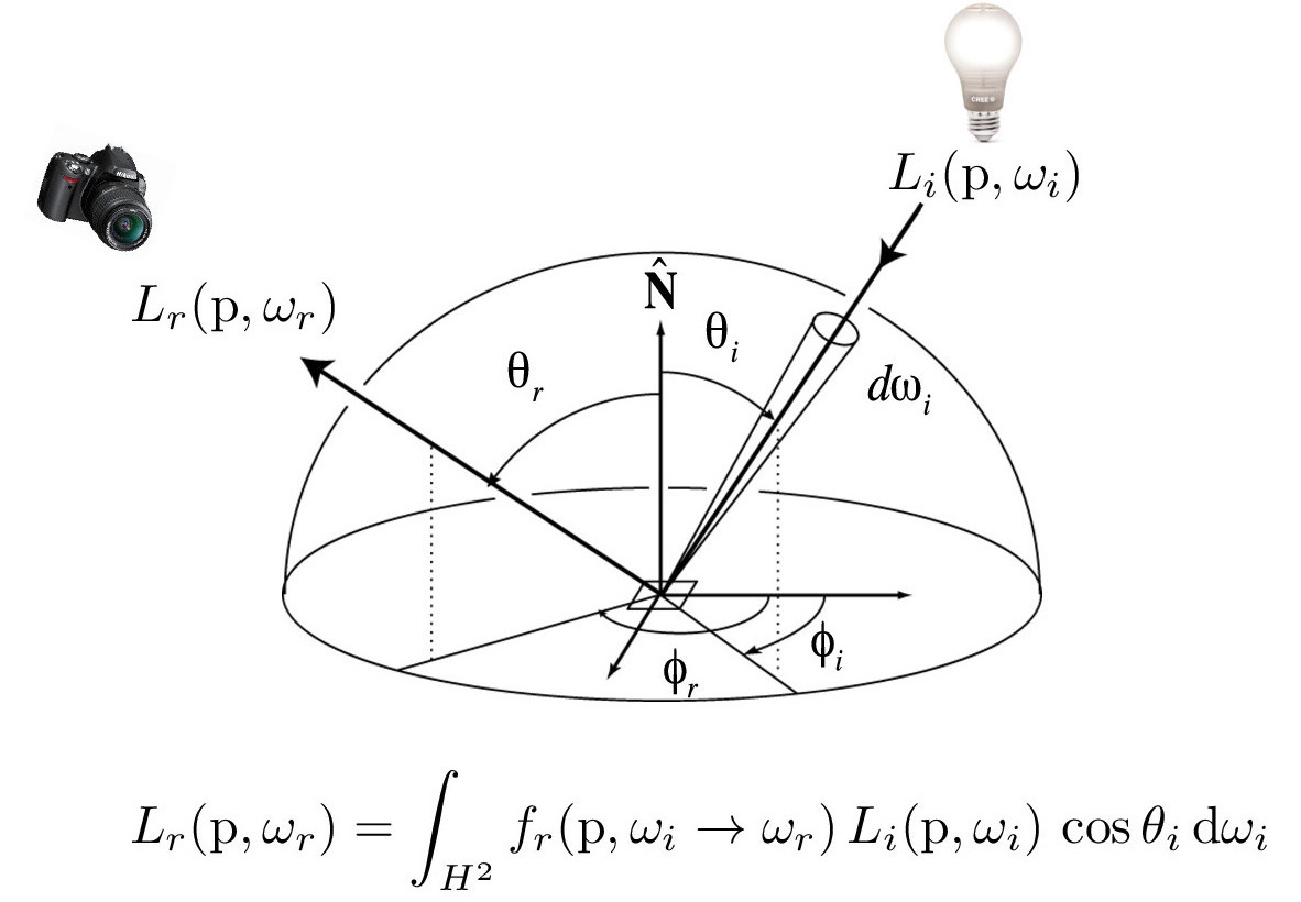
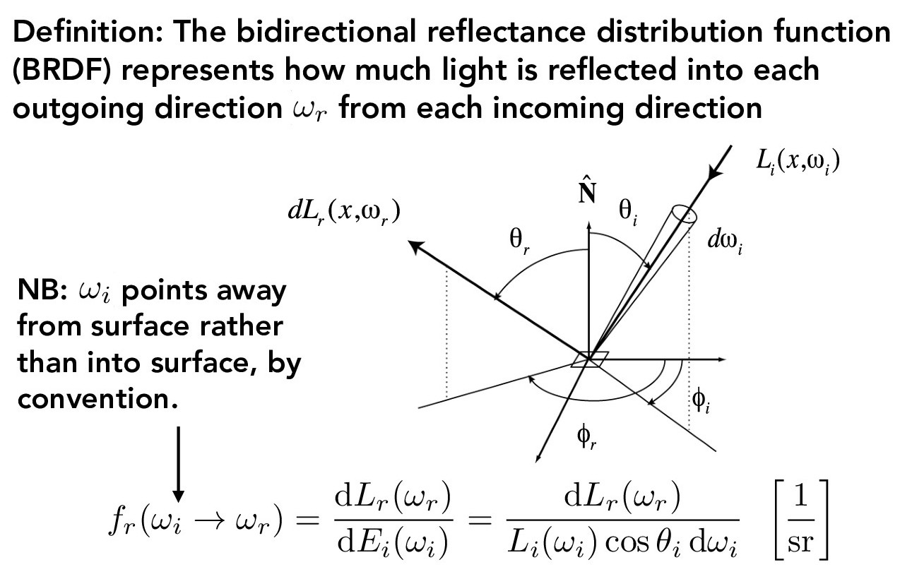
Credit: CS184/284A Lecture 13 Slides by Ren Ng

The Monte Carlo estimator of the Reflectance Equation is

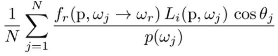
Now that we have an expression that we can use to estimate the outgoing light, we can compute the one bounce radiance. There are two ways to do this: hemisphere sampling and importance light sampling.

Hemisphere sampling, as the name implies, takes samples over the entire hemisphere. If a sample ray (starting at the intersection point \(p\) (in Fig. 3.2)) happens to intersect a light (i.e. the sample ray is not in a shadow), then we calculate the incoming light. The pseudocode is outlined below.

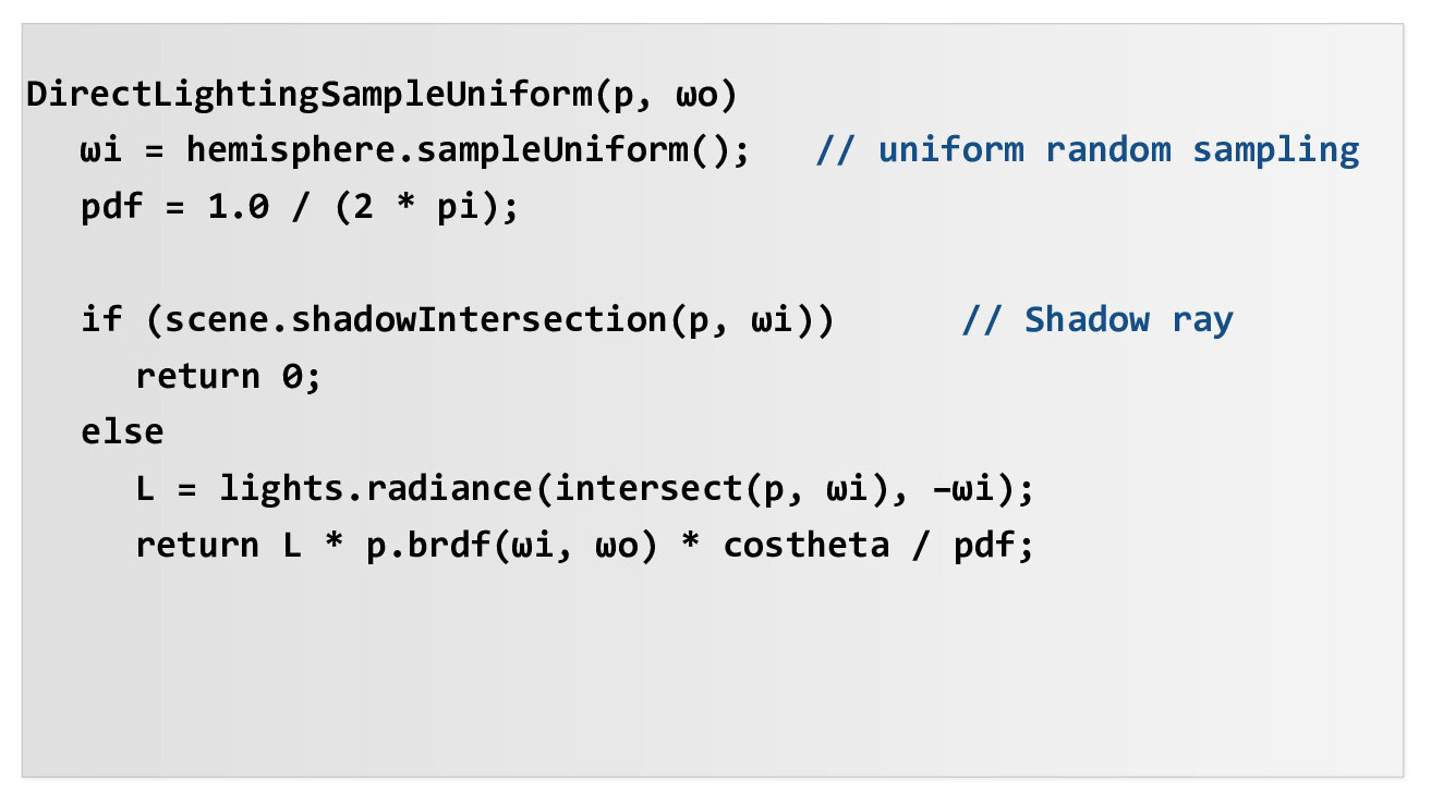
Credit: CS184/284A Lecture 13 Slides by Ren Ng

A different, more efficient approach is importance light sampling, which loops over the lights in the scenes and takes samples for each light. This way, if the sample ray is not occluded, it is guaranteed to point at a light and contribute to the overall radiance. This was not the case with hemisphere sampling, where only some of the sample directions point toward the lights. The benefit of importance light sampling is that there is less noise and less rays are needed to produce a decent result.

Here is a comparison of hemisphere and importance light sampling. Notice the noise levels of each method.

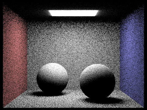
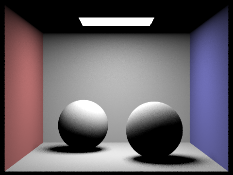
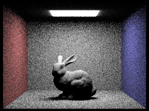
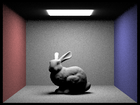
From these rendered results, we can tell that importance light sampling produces much less noise. With 16 samples per pixel and 8 per light, hemisphere sampling results in an unacceptable amount of noise. Meanwhile, importance light sampling produces an acceptable relatively noise free result and is even better than hemisphere sampling at 64 samples per pixel and 32 per light. The result of importance sampling at 64/32 samples per pixel/light looks similar to its result with 16/8 samples per pixel/light. This means we can suffice with less samples per pixel/light while still achieving a satisfactory result, which is good news for rendering times.

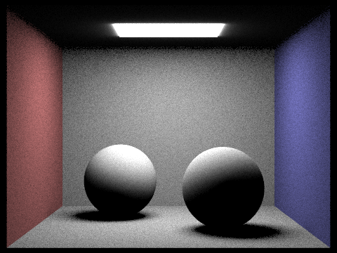
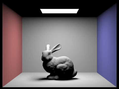
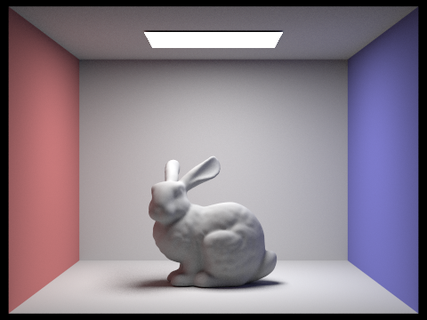
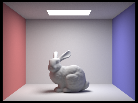
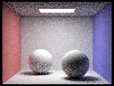
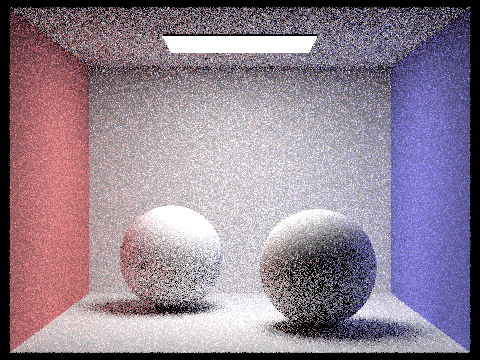
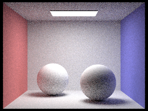
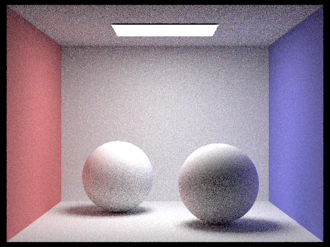
We can also compare the levels of noise for different numbers of samples per light using importance light sampling. The images below are rendered with 1 sample per pixel and varying numbers of samples per light.

Part 4: Global Illumination

In real life, light is reflected off all sorts of surfaces before reaching our eye. To create richer renders, we render scenes with global illumination, which requires us to implement indirect lighting. Indirect lighting traces multi-bounce rays, as shown below.

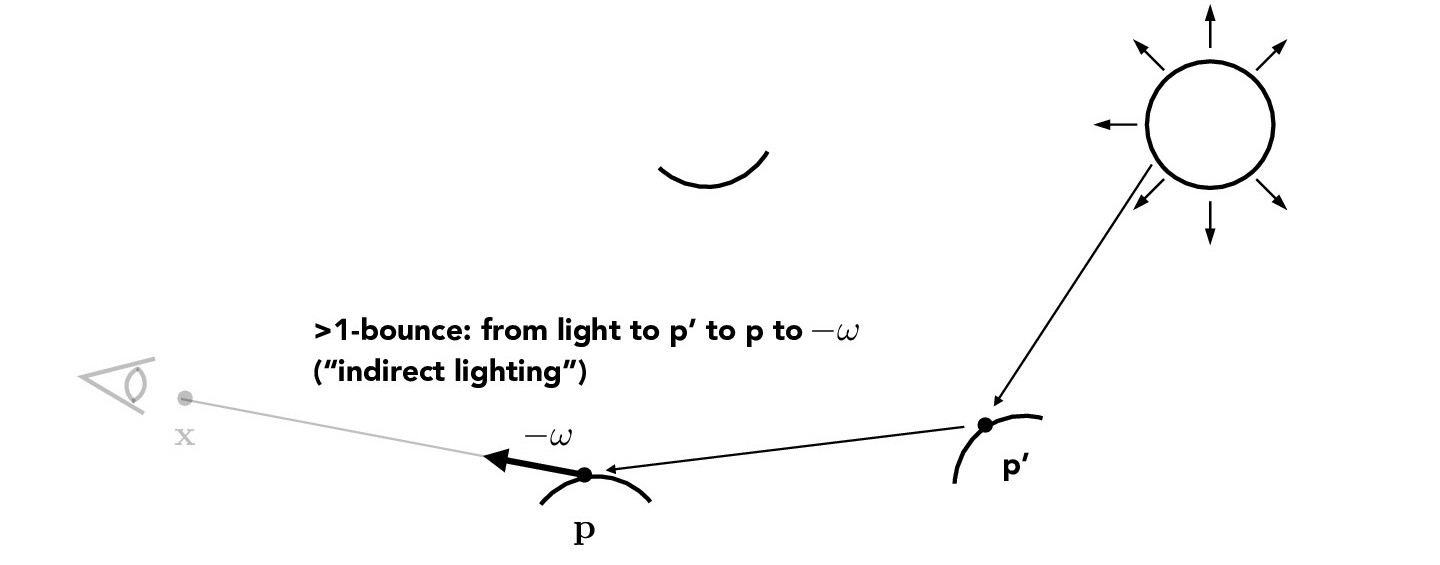
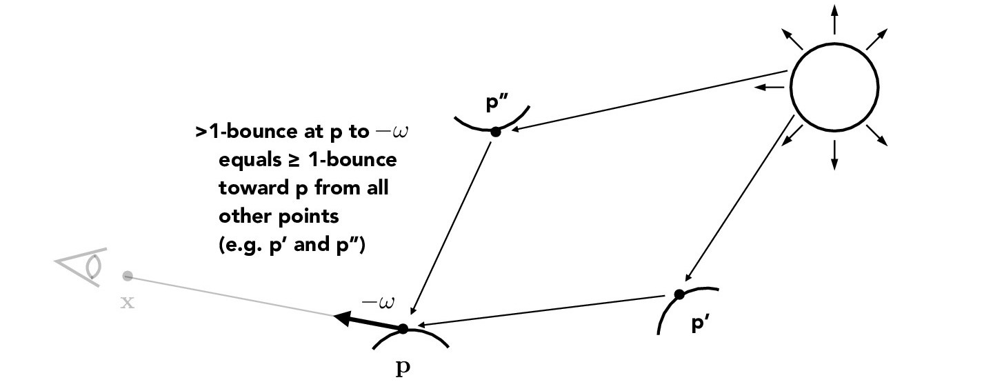
Credit: CS184/284A Lecture 13 Slides by Ren Ng

We will have an at_least_one_bounce_radiance function that is recursive to simulate one bounce, two bounces, three bounces, etc. In order to prevent infinite recursion, we use Russian Roulette and a max_ray_depth argument.

Russian roulette gives us an unbiased method of random termination. This involves a continuation probability (e.g. 0.65 but can be arbitrary). Every function call, we decide whether to keep recursing according to this continuation probability.

The max_ray_depth argument is also used to prevent infinite recursion. If max_ray_depth = 0, we return zero-bounce radiance. If max_ray_depth = 1, we return one-bounce radiance (i.e. direct lighting). If max_ray_depth > 1, we trace a maximum of max_ray_depth bounces, but we will always trace the first indirect bounce regardless of Russian Roulette.

Below is the outline of the global illumination pseudocode.

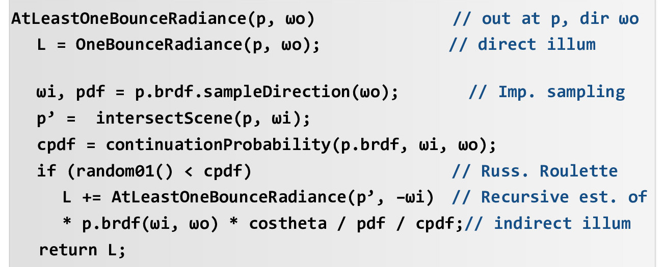
Credit: CS184/284A Lecture 13 Slides by Ren Ng

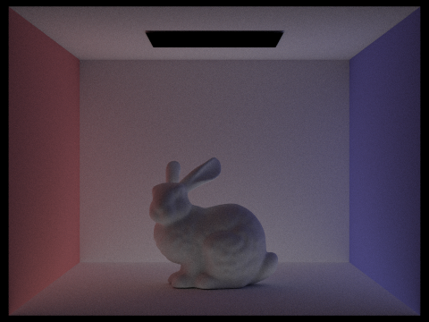
With 1024 samples per pixel, 1 sample per light, max_ray_depth = 100, the following shows the decomposition of global illumination (direct and indirect lighting).

We can also visualize how changing max_ray_depth affects our renders. The renders below each use 1024 samples per pixel and 1 sample per light. We see that the renders progressively get visually richer and more "realistic".

Now, let's compare the noise levels for global illumination depending on the number of samples per pixel. Each of the following renders used 4 samples per light and max_ray_depth = 5. As expected, noise levels decrease as sample numbers increase.

Here are a couple more examples rendered with global illumination, with 1024 samples per pixel, 4 samples per light, and max_ray_depth = 5.

Part 5: Adaptive Sampling

In the previous parts, we traced a fixed number of sample rays for each pixel. In other words, the sampling rate was uniform over the entire image. Some pixels can converge at lower sampling rates however, so it's unnecessary to sample these pixels at a high rate. Adaptive sampling concentrates more samples at the difficult parts of the image.

The algorithm we implement here will be based on individual pixel statistics. We will keep a running sum (\(s_1\)) of the samples' illuminances and a running sum (\(s_2\)) of the samples' squared illuminances. The samplesPerBatch argument indicates how often we want to check a pixel's convergence. Every samplesPerBatch iterations of the sampling loop, we check if the pixel has converged or not. This involves first calculating the mean and variance of the samples: $$\mu = \frac{s_1}{n}$$ $$\sigma^2 = \frac{1}{n - 1} \cdot \Big( s_2 - \frac{s_1^2}{n} \Big) $$ where \(n\) is the number of rays we have traced so far. The pixel convergence heuristic is given by $$ I = 1.96 \cdot \frac{\sigma}{\sqrt{n}} $$ where the \(1.96\) factor comes from a 95% confidence interval. Essentially, we want to say with 95% confidence that the average illuminance of the pixel is between \(\mu - I\) and \(\mu + I\). Then, the condition $$I \leq \text{maxTolerance} \cdot \mu$$ determines if the pixel has converged or not. If so, we break out of the sampling loop and stop tracing rays. If not, we continue sampling and tracing rays.

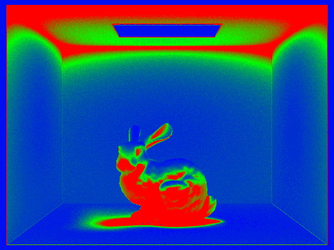
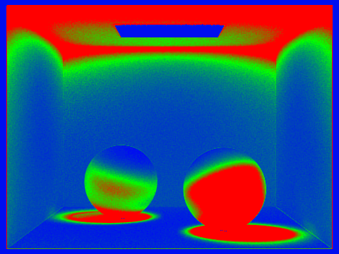
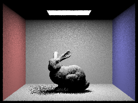
From the sampling rate images below, we can see adaptive sampling at work. The red regions represent high sampling rates while the blue regions represent low sampling rates. Both examples below use (a maximum of) 2048 samples per pixel, 1 sample per light, max_ray_depth = 5, a samplesPerBatch size of 64 and maxTolerance = 0.05.