Overview
Rasterization
Drawing Single-Color Triangles
Antialiasing by Supersampling
Transforms
Sampling
Barycentric Coordinates
"Pixel Sampling" for Texture Mapping
"Level Sampling" with Mipmaps for Texture Mapping
The goal of this project is to implement a simple rasterizer that can draw triangles, perform supersampling, perform hierarchical transforms, and texture map with antialiasing. This project reinforced my understanding of the rasterization pipeline and general concepts relating to sampling.
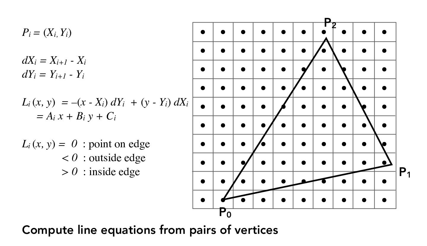
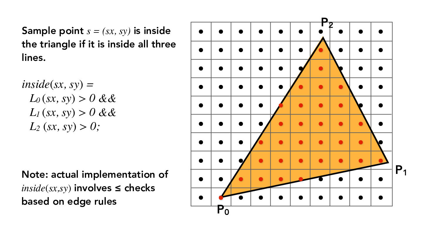
In this part, we want to rasterize a triangle with a single color. For now, we will have 1 sample per pixel. The main challenge is to determine if a pixel is within the triangle or not. Since a triangle is the intersection of three half-planes and its three vertices can define three lines, we can check that the point is in the triangle by simply checking that is on the same side of each of the triangle's edges. The following figures describe the mathematical formulae used for the point-in-triangle test.
Credit: CS184/284A Lecture 2 Slides by Ren Ng
To make our code more efficient, instead of performing a point-in-triangle test for all pixels in the framebuffer, we will only search within the bounding box of the triangle. For example, in the figures above, the boundary of the grid is the bounding box, and we would perform point-in-triangle tests for each sample in the grid (black dots).
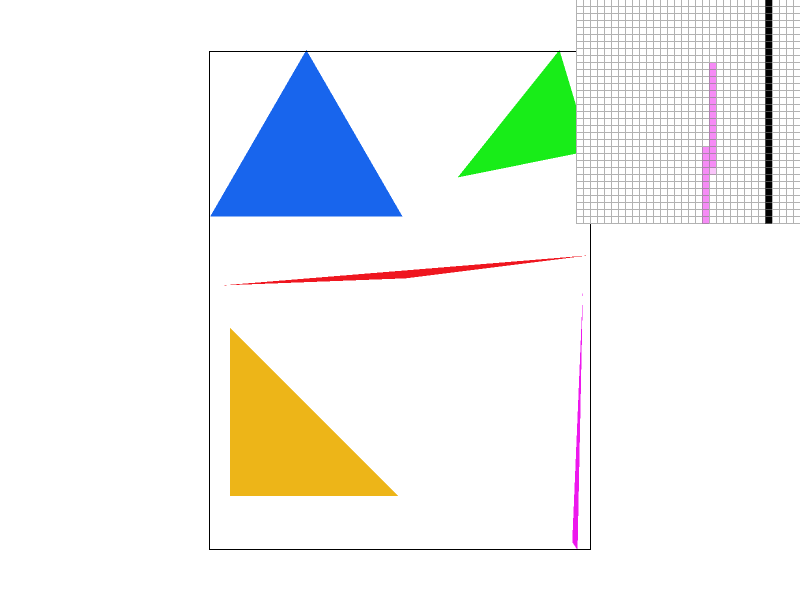
The following are several examples using the above method:
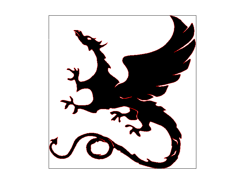
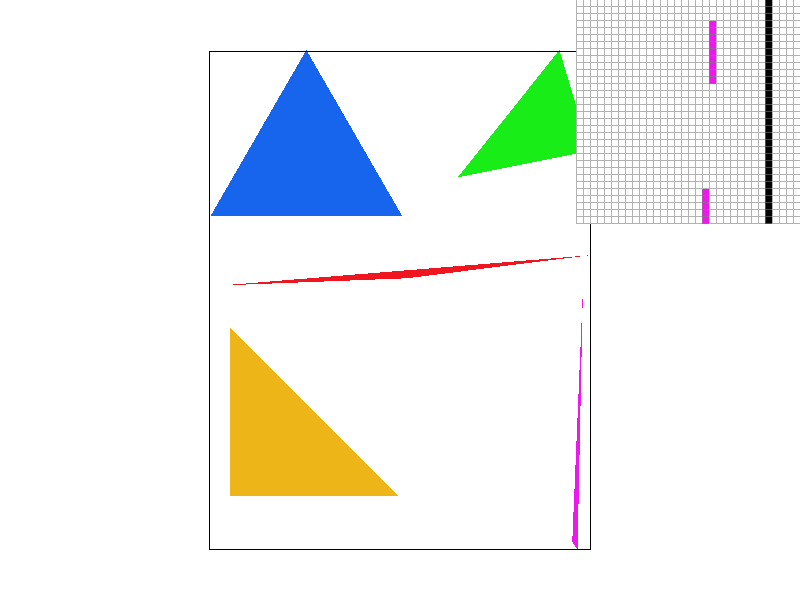
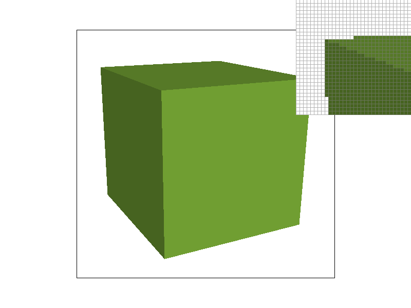
Notice that in "svg4" the skinny pink triangle is disconnected, and in "svg5", the edges of the cube are jagged. This is due to aliasing.
As shown in the previous part, some of our results were aliased. Supersampling will allow us to perform antialiasing. This means we will sample multiple locations within a pixel and average their values. Supersampling approximates the effect of a 1-pixel box filter, filtering out high frequencies.
The supersampling algorithm is similar to the method from the previous part. The main difference is that instead of sampling 1 time per pixel, we will uniformly sample N x N (= sampling rate) times per pixel. This effectively increases the resolution of our image. Since we have a lot more information to keep track of than in the sampling rate=1 case, we will need an array (which we will call the sample_buffer) that stores the color information of all our samples. Once we have filled the sample_buffer with all the data we need, to resolve the sample_buffer to the framebuffer (i.e. downsample the sample_buffer to fit the resolution of the framebuffer), we average the colors of each pixel's N x N samples. The following figures illustrate this averaging process.
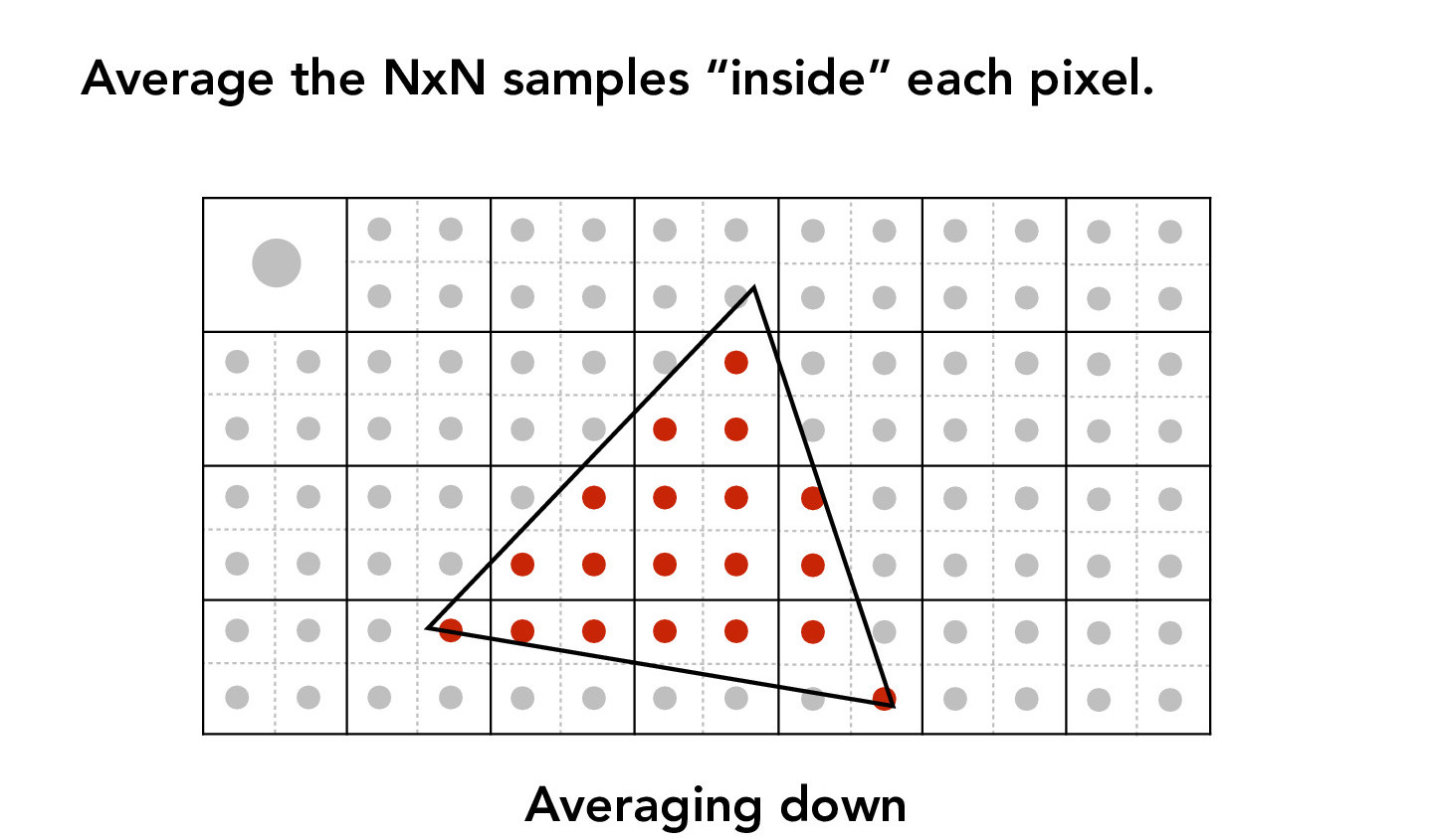
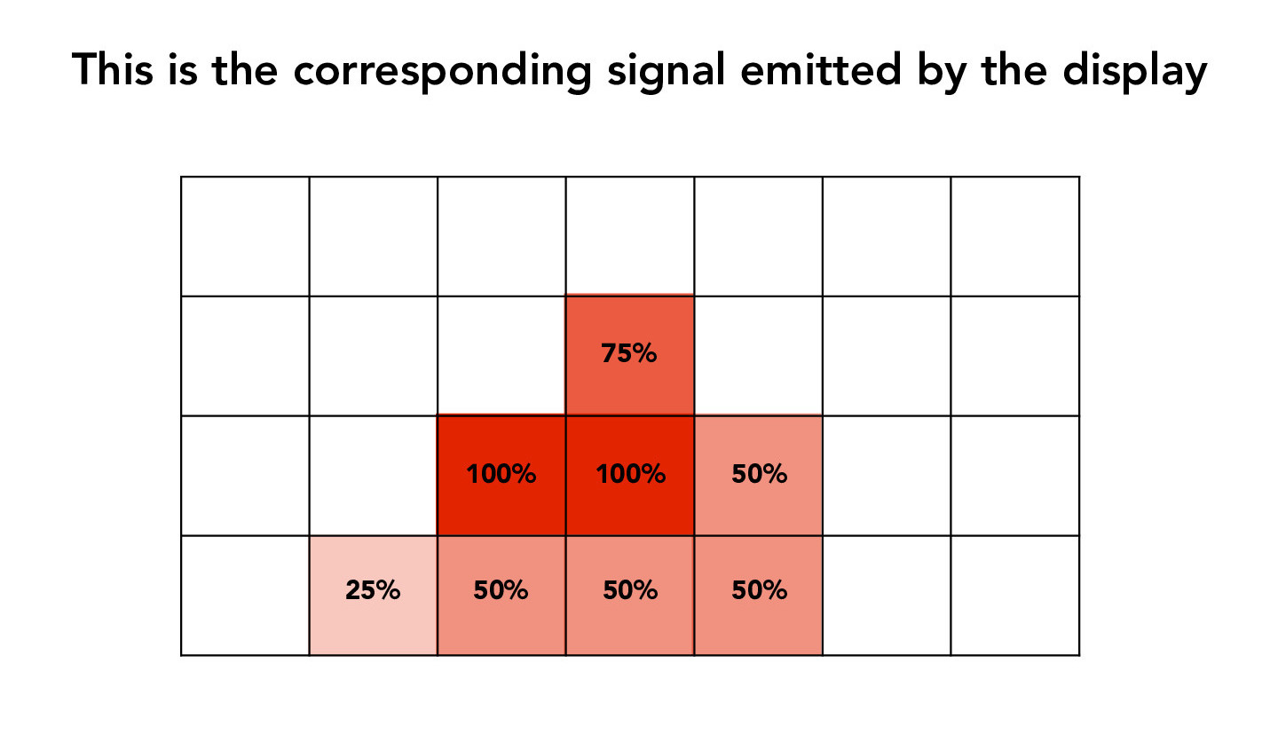
Credit: CS184/284A Lecture 3 Slides by Ren Ng
The result will have less jaggies (jagged/pixelated edges). We can see this from the examples below. As the sampling rate is increased, the result becomes "smoother" and less aliased. Notice that for the skinny pink triangle, it is no longer disconnected when sampled at higher sampling rates. This is one example of how supersampling (and antialiasing in general) can be useful.


Affine transformations (e.g. translation, scale, rotation) can be expressed in 3x3 matrices using homogeneous coordinates.
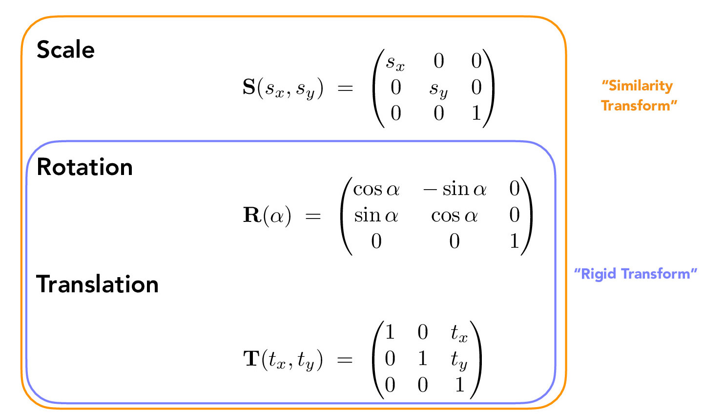
Credit: CS184/284A Lecture 4 Slides by Ren Ng
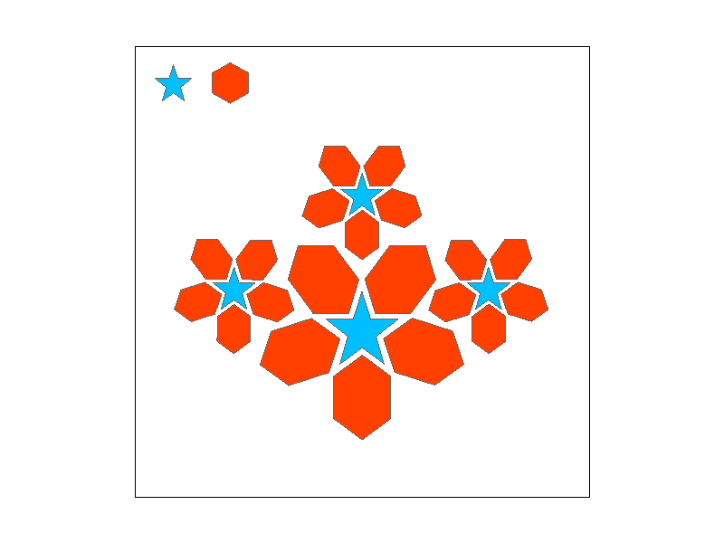
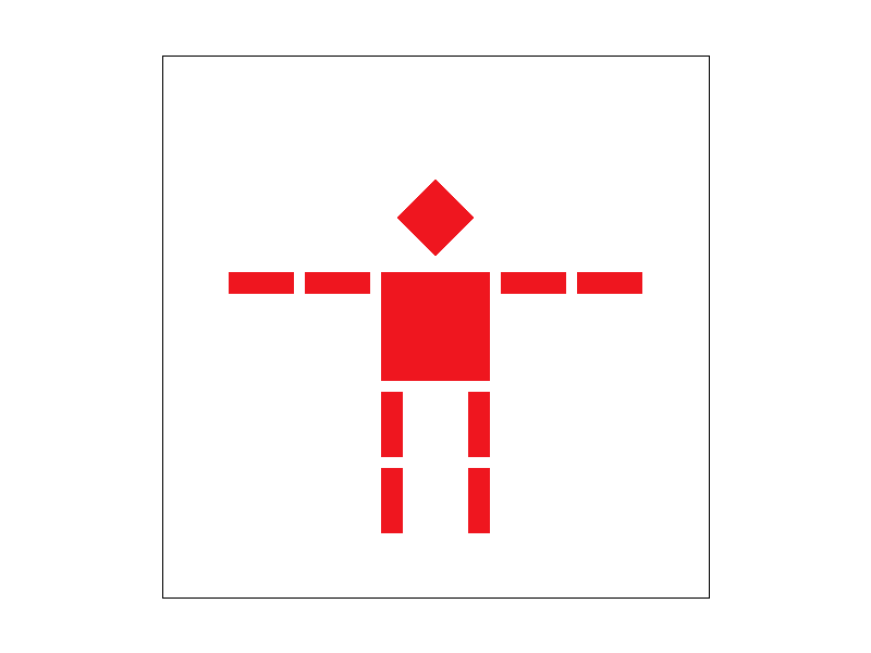
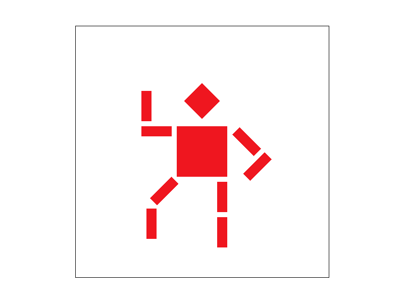
A sequence of transformations are applied to various shapes in the following images to pose a robot. The order of transformation matters because matrix multiplication is not commutative. We are also able to hierarchically transform the shapes and transform multiple shapes at once.
Barycentric coordinates are a coordinate system to express points in a triangle (in the 2D case.) Each point in the triangle is expressed with (alpha, beta, gamma); each of these values represents the proportional distance of a point and a vertex to the vertex's opposite edge. The left figure below illustrates this idea. The right figure details how to compute the barycentric coordinates of a point (x, y).
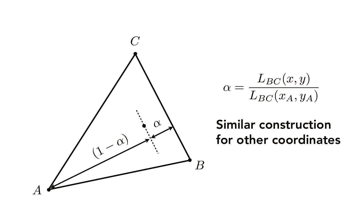
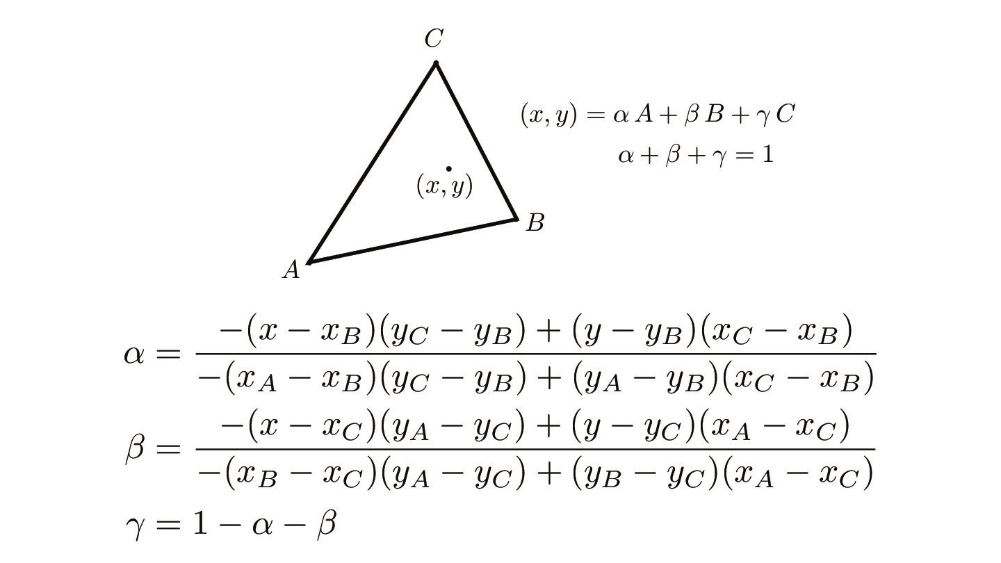
Credit: CS184/284A Lecture 5 Slides by Ren Ng
Barycentric coordinates have many use cases. As shown below, we can use barycentric coordinates to interpolate color. Each vertex V_A, V_B, and V_C represents an RGB color, and the color for each point in the interior of the triangle is then defined as a function of its barycentric coordinates. This will be helpful when we implement texture mapping (in the following parts).
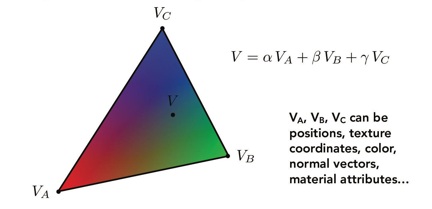
Credit: CS184/284A Lecture 5 Slides by Ren Ng
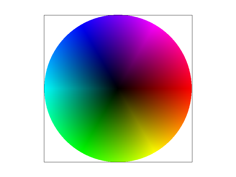
The following is another example that uses barycentric coordinates to interpolate color.
Previously, we could color triangles with a solid color or with a gradient. Now, suppose we want triangles with different patterns or images. This requires us to sample from a texture map. When we map a texture onto a triangle, we need to sample from the texture space to retrieve the color we want to display. The barycentric coordinates of a point can be used in both the xy screen space and uv texture space, but the screen space and texture space may not be one-to-one mappings. In other words, each screen pixel sample may not correspond to one texel (texture pixel). We then need texture filtering techniques in order to calculate the sample colors from the texels. Nearest neighbor and bilinear interpolation are two commonly-used methods.
Nearest neighbor interpolation finds the closest texel to sample from. Meanwhile, bilinear interpolation looks at the four neighboring texels and interpolates their colors. The diagram below shows more information.
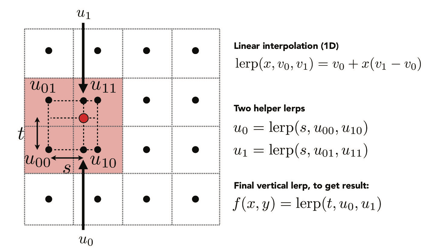
Credit: CS184/284A Lecture 5 Slides by Ren Ng
In both methods, if a texture coordinate lies outside of the texture, we clamp it.
Here are the results of the texture-mapped Berkeley seal using the two different interpolation methods and at different sampling rates.
Notice how bilinear interpolation is better at antialiasing than nearest neighbor interpolation.

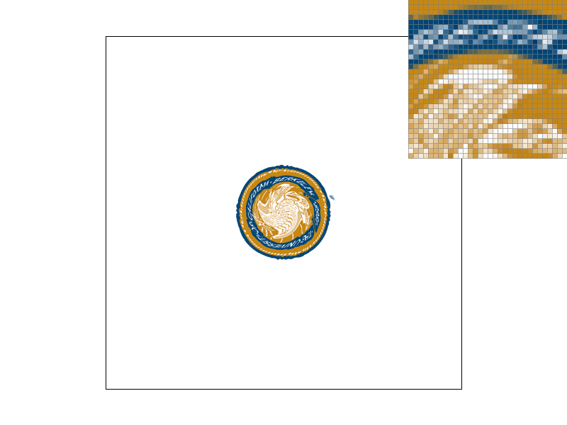


Pixel sampling is oftentimes not enough to produce a satisfactory result. Using one image to texture map a scene may cause aliasing in some areas. And if the texture is downsampled to resolve the aliasing, it may cause blurring in other areas. This is illustrated below.
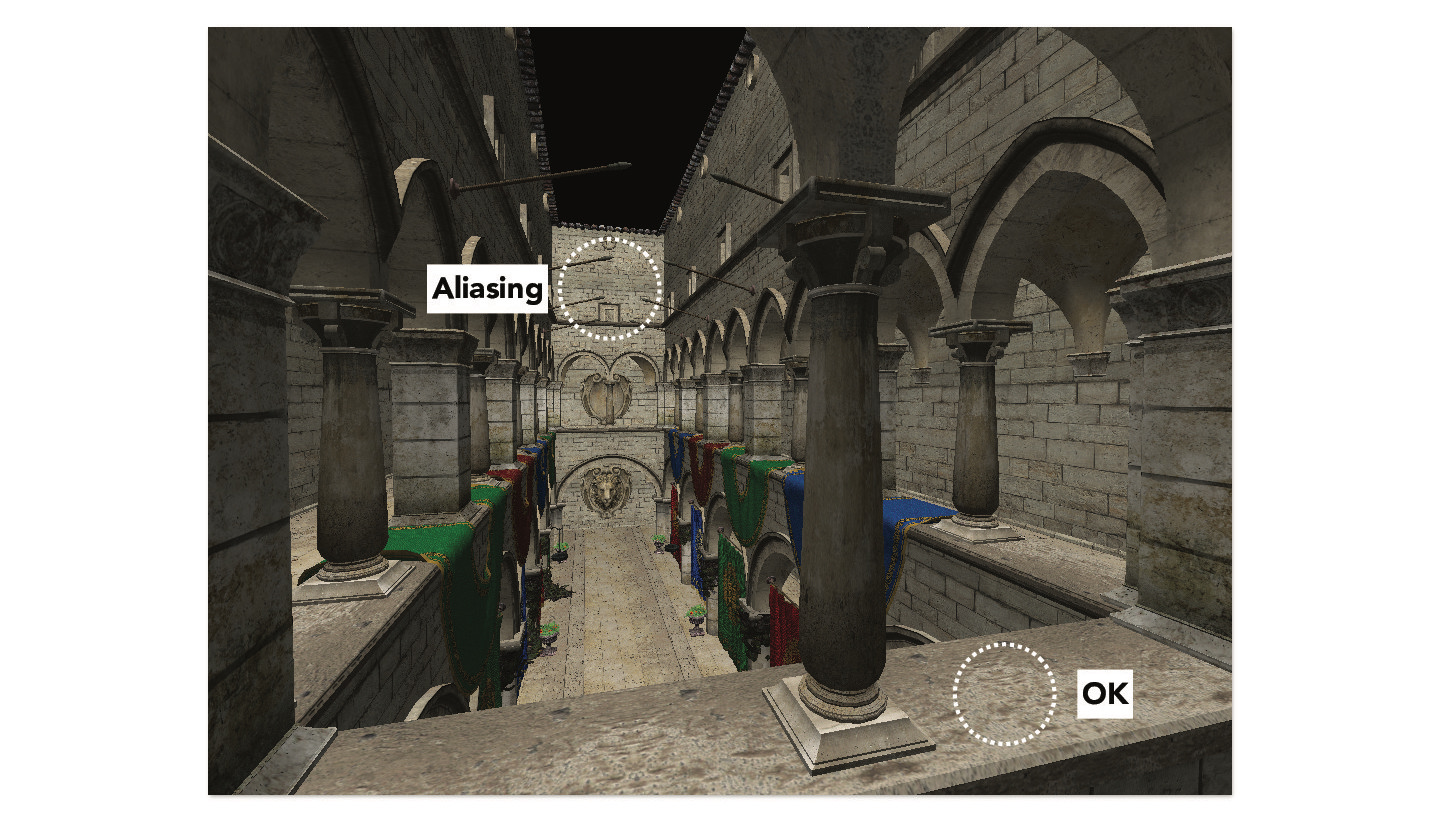
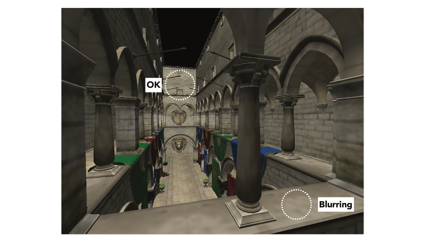
Credit: CS184/284A Lecture 5 Slides by Ren Ng
The solution is to use level sampling, which is to sample from multiple images—more specifically, the same texture but at different resolutions. This sequence of images is known as a mipmap (i.e. image pyramid); at each level of the mipmap, the image is a lower resolution version of the level below's. The level 0 image is at the original resolution; higher levels are at progressively lower resolutions. The following images show the different levels of a mipmap.
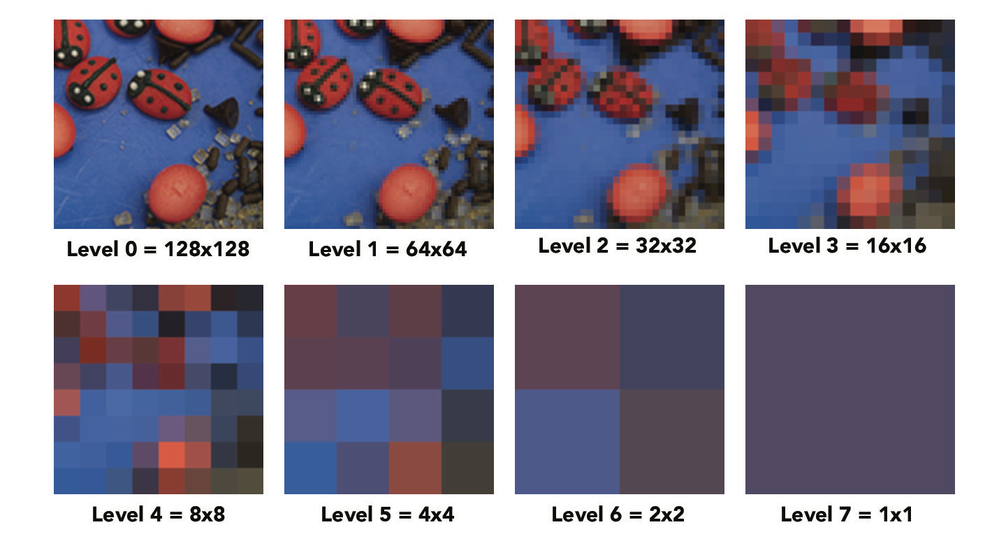
Credit: CS184/284A Lecture 5 Slides by Ren Ng
In this part, we will implement three different level sampling methods: zero, nearest neighbor, and bilinear. For the "zero" method, we simply sample from the zero-th level of the mipmap.
For the nearest neighbor and bilinear level sampling methods, we need to determine the appropriate mipmap level from which to sample. The first step is to calculate the partial derivatives of the (u, v) texture coordinates with respect to x and y. Then, using the formula shown below, we can calculate L (the length in pixels in the original image) and then D (the mipmap level). The larger L is, the lower the resolution we want to sample from.
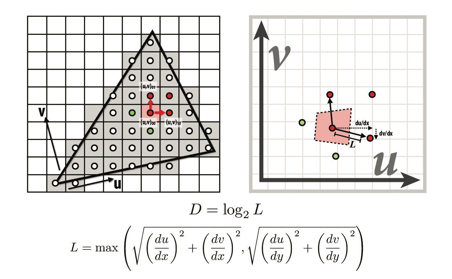
Credit: CS184/284A Lecture 5 Slides by Ren Ng
In nearest neighbor level sampling, we sample from the nearest mipmap level (round D value to an integer). If the level D value is invalid, we will clamp it. For bilinear level sampling, we sample from adjacent levels (floor and ceiling of D) and linearly interpolate. When both bilinear pixel sampling and bilinear level sampling are used, it is known as trilinear sampling.
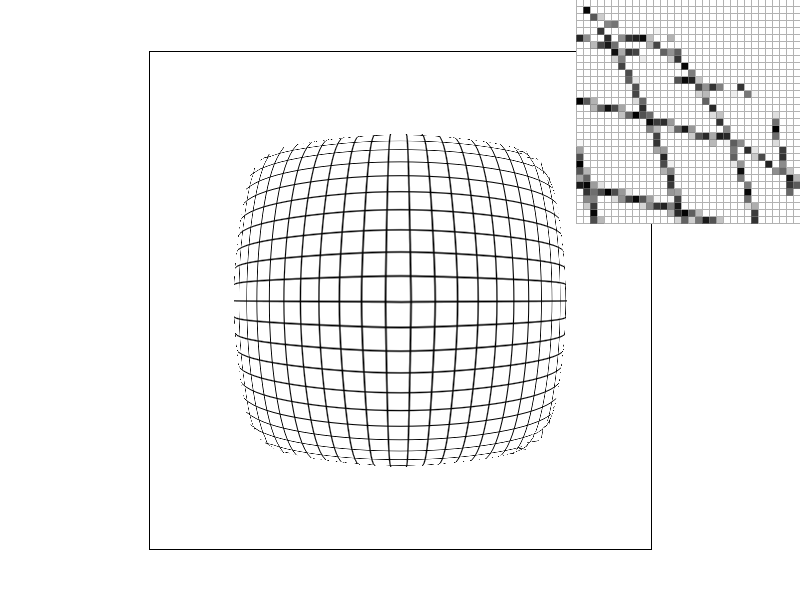
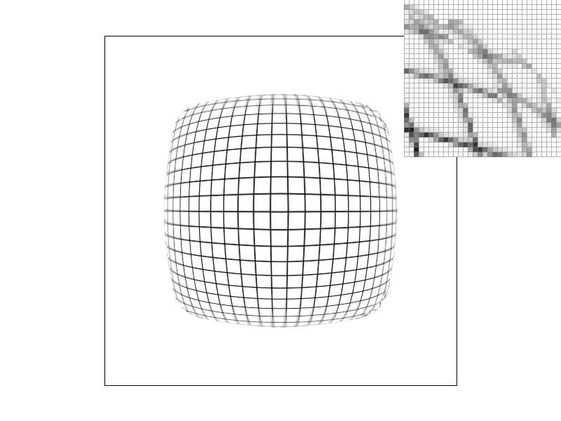
Below are examples of warped grid and brick textures using the different level and pixel sampling methods.


Brick texture:


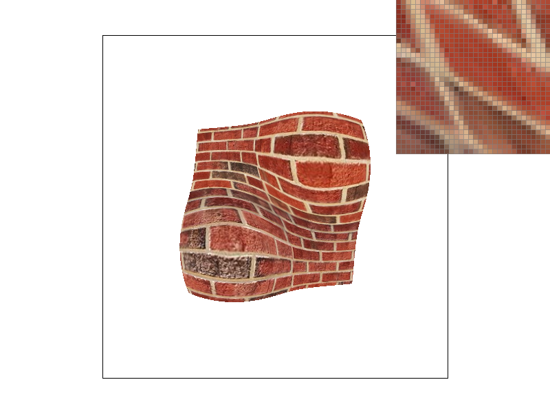

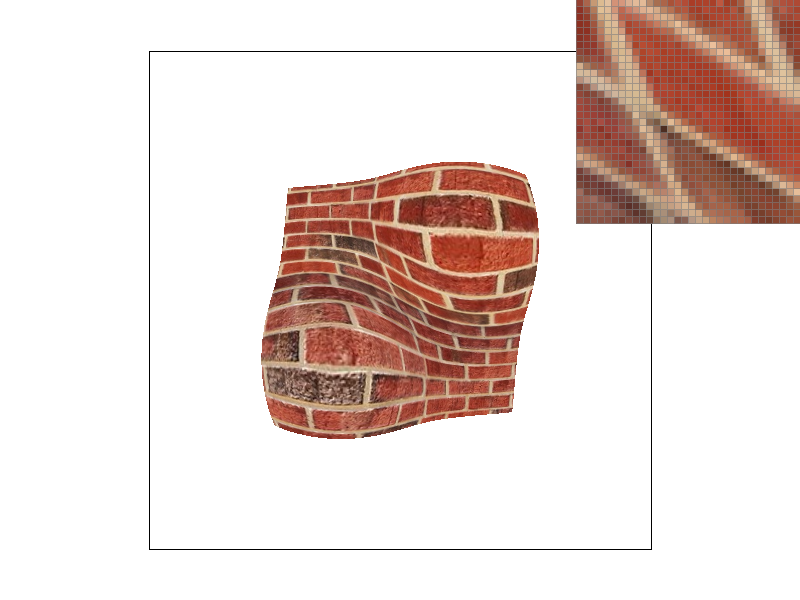
In both the grid and brick examples, we can see the effect that the different pixel and level sampling techniques have on antialiasing.
Now that we have implemented three sampling techniques: supersampling, pixel sampling, and level sampling, let's compare the different tradeoffs of speed, memory usage, and antialiasing power. Supersampling is costly, both in terms of speed and memory usage. In comparison, pixel sampling is faster and uses less memory. As was mentioned previously however, pixel sampling sometimes sacrifices detail for antialiasing and vice versa. Level sampling is also faster and uses less memory than supersampling. And not only this, but it also has the most antialiasing power of the three sampling techniques. Level sampling solves the issue with pixel sampling; it antialiases appropriately while preserving detail where needed.